


m →Other websites: Add {{source}} tag |
revise |
||
| (3 intermediate revisions by 2 users not shown) | |||
| Line 1: | Line 1: | ||
{{ | {{Short description|Study of collection and analysis of data}} | ||
{{hatnote group| | |||
{{about|the study of data|a value derived from a sample|Statistic}} | |||
{{Other uses|Statistics (disambiguation)}} | |||
}} | |||
[[File:Standard Normal Distribution-en.svg|thumb|upright=1.3|right|The [[normal distribution]], a very common [[Probability density function|probability density]], is used extensively in [[inferential statistics]].]] | |||
[[File:Iris Pairs Plot.svg|thumb|upright=1.3|right|[[Scatter plot]]s and [[line chart]]s are used in [[descriptive statistics]] to show the observed relationships between different variables, here using the [[Iris flower data set|''Iris'' flower data set]].]] | |||
{{StatsTopicTOC}} | |||
{{Math topics TOC}} | |||
<!--PLEASE DO NOT EDIT THE OPENING SENTENCE WITHOUT FIRST PROPOSING YOUR CHANGE AT THE TALK PAGE.--> | |||
'''Statistics''' (from [[German language|German]]: ''{{linktext|lang=de|Statistik}}'', {{Abbr|orig.|originally}} "description of a [[State (polity)|state]], a country"<ref name=":1">{{multiref | {{Cite OED|statistics}} | {{Cite encyclopedia |encyclopedia=Digitales Wörterbuch der deutschen Sprache |url=https://www.dwds.de/?q=Statistik |title=Statistik | date=August 2024 |publisher=Berlin-Brandenburgischen Akademie der Wissenschaften |lang=de}} }}</ref>) is the discipline that concerns the collection, organization, analysis, interpretation, and presentation of [[data]].<ref name="def">{{multiref | {{Cite encyclopedia |encyclopedia=Oxford Reference |title=Statistics |year=2008 |publisher=Oxford University Press |isbn=978-0-19-954145-4 |url=https://www.oxfordreference.com/view/10.1093/acref/9780199541454.001.0001/acref-9780199541454-e-1566?rskey=nxhBLl&result=1979}} | {{Cite encyclopedia |first=Jan-Willem |last=Romijn |year=2014 |title=Philosophy of statistics |encyclopedia=Stanford Encyclopedia of Philosophy |url=http://plato.stanford.edu/entries/statistics/}} | {{Cite dictionary | dictionary=Cambridge Dictionary |title=Statistics |url=https://dictionary.cambridge.org/dictionary/english/statistics}} }}</ref> In applying statistics to a scientific, industrial, or social problem, it is conventional to begin with a [[statistical population]] or a [[statistical model]] to be studied. Populations can be diverse groups of people or objects such as "all people living in a country" or "every atom composing a crystal". Statistics deals with every aspect of data, including the planning of data collection in terms of the design of [[statistical survey|surveys]] and [[experimental design|experiments]].<ref name="Dodge">{{Cite book |last=Dodge |first=Yadolah |title=The Oxford Dictionary of Statistical Terms |publisher=Oxford University Press |year=2003 |isbn=0-19-920613-9}}</ref> Statistics is deeply related to subjects like physics, chemistry, geography, geopolitics, and especially mathematics. | |||
When [[census]] data (comprising every member of the target population) cannot be collected, [[statistician]]s collect data by developing specific experiment designs and survey [[sample (statistics)|samples]]. Representative sampling assures that inferences and conclusions can reasonably extend from the sample to the population as a whole. An [[experimental study]] involves taking measurements of the system under study, manipulating the system, and then taking additional measurements using the same procedure to determine if the manipulation has modified the values of the measurements. In contrast, an [[observational study]] does not involve experimental manipulation. | |||
Two main statistical methods are used in [[data analysis]]: [[descriptive statistics]], which summarize data from a sample using [[Index (statistics)|indexes]] such as the [[mean]] or [[standard deviation]], and [[statistical inference|inferential statistics]], which draw conclusions from data that are subject to random variation (e.g., observational errors, sampling variation).<ref name=LundResearchLtd>{{cite web |last=Lund Research Ltd. |url=https://statistics.laerd.com/statistical-guides/descriptive-inferential-statistics.php |title=Descriptive and Inferential Statistics |publisher=statistics.laerd.com |access-date=2014-03-23 |archive-date=2020-10-26 |archive-url=https://web.archive.org/web/20201026075549/https://statistics.laerd.com/statistical-guides/descriptive-inferential-statistics.php |url-status=live }}</ref> Descriptive statistics are most often concerned with two sets of properties of a ''distribution'' (sample or population): ''[[central tendency]]'' (or ''location'') seeks to characterize the distribution's central or typical value, while ''[[statistical dispersion|dispersion]]'' (or ''variability'') characterizes the extent to which members of the distribution depart from its center and each other. Inferences made using [[mathematical statistics]] employ the framework of [[probability theory]], which deals with the analysis of random phenomena. | |||
A standard statistical procedure involves the collection of data leading to a [[statistical hypothesis testing|test of the relationship]] between two statistical data sets, or a data set and synthetic data drawn from an idealized model. A hypothesis is proposed for the statistical relationship between the two data sets, an [[alternative hypothesis|alternative]] to an idealized [[null hypothesis]] of no relationship between two data sets. Rejecting or disproving the null hypothesis is done using statistical tests that quantify the sense in which the null can be proven false, given the data that are used in the test. Working from a null hypothesis, two basic forms of error are recognized: [[Type I error]]s (null hypothesis is rejected when it is in fact true, giving a "false positive") and [[Type II error]]s (null hypothesis fails to be rejected when it is in fact false, giving a "false negative"). Multiple problems have come to be associated with this framework, ranging from obtaining a sufficient sample size to specifying an adequate null hypothesis.<ref name="LundResearchLtd" /> | |||
Statistical measurement processes are also prone to error with regard to the data they generate. Many of these errors are classified as random (noise) or systematic ([[Bias (statistics)|bias]]), but other types of errors (e.g., blunder, such as when an analyst reports incorrect units) can also occur. The presence of [[missing data]] or [[censoring (statistics)|censoring]] may result in biased estimates, and specific techniques have been developed to address these problems. | |||
{{TOC limit|3}} | |||
== Introduction == | |||
{{main|Outline of statistics}} | |||
{{blockquote|"Statistics is both the science of uncertainty and the technology of extracting information from data." - featured in the International Encyclopedia of Statistical Science.<ref name="Hand20102">{{Cite book |last=Hand |first=David |title=International Encyclopedia of Statistical Science |publisher=Springer |year=2010 |isbn=978-3-642-04898-2 |editor-last=Lovric |editor-first=Miodrag |pages=1504–1509 |language=en |chapter=Statistics: An Overview}}</ref>}}Statistics is the discipline that deals with [[data]], facts and figures with which meaningful information is inferred. Data may represent a numerical value, in form of quantitative data, or a label, as with qualitative data. Data may be collected, presented and summarised, in one of two methods called descriptive statistics. Two elementary summaries of data, singularly called a statistic, are the mean and dispersion. Whereas inferential statistics interprets data from a population sample to induce statements and predictions about a population.<ref>{{Cite book |last=Tanton |first=James |title=Encyclopedia of Mathematics |publisher=Facts On File |year=2005 |isbn=0-8160-5124-0 |pages=478–484 |language=en |chapter=Statistics}}</ref><ref name=":2">{{Cite web |date=2024-12-06 |title=Statistics {{!}} Definition, Types, & Importance {{!}} Britannica |url=https://www.britannica.com/science/statistics |access-date=2024-12-30 |website=www.britannica.com |language=en}}</ref><ref name="Hand20102" /> | |||
Statistics is regarded as a body of science<ref name="Moses">Moses, Lincoln E. (1986) ''Think and Explain with Statistics'', Addison-Wesley, {{isbn|978-0-201-15619-5}}. pp. 1–3</ref> or a branch of mathematics.<ref>Hays, William Lee, (1973) ''Statistics for the Social Sciences'', Holt, Rinehart and Winston, p. xii, {{isbn|978-0-03-077945-9}}</ref> It is based on probability, a branch of mathematics that studies random events. Statistics is considered the science of uncertainty. This arises from the ways to cope with measurement and sampling error as well as dealing with uncertanties in modelling. Although probability and statistics were once paired together as a single subject, they are conceptually distinct from one another. The former is based on deducing answers to specific situations from a general theory of probability, meanwhile statistics induces statements about a population based on a data set. Statistics serves to bridge the gap between probability and applied mathematical fields.<ref>{{Cite book |last=Williams |first=David |title=Weighing the Odds: A Course in Probability and Statistics |publisher=Cambridge University Press |year=2001 |isbn=9780521006187 |pages=xi-xvii |language=en |chapter=Preface}}</ref><ref name="Hand20102" /><ref>{{Cite book |last=Rudas |first=Tamas |title=International Encyclopedia of Statistical Science |publisher=Springer |year=2010 |isbn=978-3-642-04898-2 |editor-last=Lovric |editor-first=Miodrag |pages=1123–1126 |language=en |chapter=Probability Theory: An Outline}}</ref> | |||
Some consider statistics to be a distinct [[Mathematical sciences|mathematical science]] rather than a branch of mathematics. While many scientific investigations make use of data, statistics is generally concerned with the use of data in the context of uncertainty and decision-making in the face of uncertainty.<ref>{{cite book |last=Moore |first=David |title=Statistics for the Twenty-First Century |publisher=The Mathematical Association of America |year=1992 |isbn=978-0-88385-078-7 |editor=F. Gordon |location=Washington, DC |pages=[https://archive.org/details/statisticsfortwe0000unse/page/14 14–25] |chapter=Teaching Statistics as a Respectable Subject |editor2=S. Gordon |chapter-url=https://archive.org/details/statisticsfortwe0000unse/page/14}}</ref><ref>{{cite book |last=Chance |first=Beth L. |author1-link=Beth Chance |title=Investigating Statistical Concepts, Applications, and Methods |author2=Rossman, Allan J. |publisher=Duxbury Press |year=2005 |isbn=978-0-495-05064-3 |chapter=Preface |access-date=2009-12-06 |chapter-url=http://www.rossmanchance.com/iscam/preface.pdf |archive-url=https://web.archive.org/web/20201122092901/http://www.rossmanchance.com/iscam/preface.pdf |archive-date=2020-11-22 |url-status=live}}</ref> Statistics is indexed at 62, a subclass of probability theory and stochastic processes, in the Mathematics Subject Classification.<ref>{{Cite web |title=Classification Search Result - zbMATH Open |url=https://zbmath.org/classification/?q=cc:62 |access-date=2024-12-30 |website=zbmath.org}}</ref> Mathematical statistics is covered in the range 276-280 of subclass QA (science > mathematics) in the Library of Congress Classification.<ref>{{Cite book |last=Higham |first=Nicholas J. |title=Handbook of Writing for the Mathematical Sciences |publisher=Society for Industrial and Applied Mathematics |year=1998 |isbn=0-89871-420-6 |pages=214 |language=en |chapter=Aids and Resources for Writing and Research}}</ref> | |||
The word statistics ultimately comes from the Latin word Status, meaning "situation" or "condition" in society, which in late Latin adopted the meaning "state". Derived from this, political scientist Gottfried Achenwall, coined the German word statistik (a summary of how things stand). In 1770, the term entered the English language through German and referred to the study of political arrangements. The term gained its modern meaning in the 1790s in John Sinclair's works.<ref>{{Cite book |last=Sheynin |first=Oscar |title=International Encyclopedia of Statistical Science |publisher=Springer |year=2010 |isbn=978-3-642-04898-2 |editor-last=Lovric |editor-first=Miodrag |pages=1493–1504 |language=en |chapter=Statistics, History of}}</ref><ref>{{Cite book |last= |first= |title=The Concise Oxford Dictionary of English Etymology |publisher=Oxford University Press |year=1996 |isbn=0-19-283098-8 |editor-last=Hoad |editor-first=T. F. |pages=460 |language=en}}</ref> In modern German, the term statistik is synonymous with mathematical statistics. The term statistic, in singular form, is used to describe a function that returns its value of the same name.<ref>{{Cite web |title=Statistik |url=https://www.spektrum.de/lexikon/mathematik/statistik/9965 |access-date=2024-12-30 |website=www.spektrum.de |language=de}}</ref> | |||
==Statistical data== | |||
=== Data collection === | |||
====Sampling==== | |||
When full census data cannot be collected, statisticians collect sample data by developing specific [[design of experiments|experiment designs]] and [[survey sampling|survey samples]]. Statistics itself also provides tools for prediction and forecasting through [[statistical model]]s. | |||
To use a sample as a guide to an entire population, it is important that it truly represents the overall population. Representative [[sampling (statistics)|sampling]] ensures that inferences and conclusions can safely be extended from the sample to the population as a whole. A major problem lies in determining the extent to which the chosen sample is actually representative. Statistics offers methods to estimate and correct for any bias in the sample and data collection procedures. There are also methods of experimental design that can lessen these issues at the outset of a study, strengthening its ability to discern truths about the population. | |||
Sampling theory is part of the [[mathematics|mathematical discipline]] of [[probability theory]]. Probability is used in [[statistical theory|mathematical statistics]] to study the [[sampling distribution]]s of [[sample statistic]]s and, more generally, the properties of [[statistical decision theory|statistical procedures]]. The use of any statistical method is valid only when the system or population under consideration satisfies the assumptions of the method. The difference in point of view between classic probability theory and sampling theory is, roughly, that probability theory starts with the given parameters of a total population to [[deductive reasoning|deduce]] probabilities that pertain to samples. Statistical inference, however, moves in the opposite direction—[[inductive reasoning|inductively inferring]] from samples to the parameters of a larger or total population. | |||
====Experimental and observational studies==== | |||
A common goal for a statistical research project is to investigate [[causality]], and in particular to draw a conclusion on the effect of changes in the values of predictors or [[Dependent and independent variables|independent variables on dependent variables]]. There are two major types of causal statistical studies: [[Experiment|experimental studies]] and [[Observational study|observational studies]]. In both types of studies, the effect of differences of an independent variable (or variables) on the behavior of the dependent variable are observed. The difference between the two types lies in how the study is actually conducted. Each can be very effective. An experimental study involves taking measurements of the system under study, manipulating the system, and then taking additional [[Level of measurement|measurements with different levels]] using the same procedure to determine if the manipulation has modified the values of the measurements. In contrast, an observational study does not involve [[Scientific control|experimental manipulation]]. Instead, data are gathered and correlations between predictors and response are investigated. While the tools of data analysis work best on data from [[Randomized controlled trial|randomized studies]], they are also applied to other kinds of data—like [[natural experiment]]s and [[Observational study|observational studies]]<ref>[[David A. Freedman (statistician)|Freedman, D.A.]] (2005) ''Statistical Models: Theory and Practice'', Cambridge University Press. {{isbn|978-0-521-67105-7}}</ref>—for which a statistician would use a modified, more structured estimation method (e.g., [[Difference in differences|difference in differences estimation]] and [[instrumental variable]]s, among many others) that produce [[consistent estimator]]s. | |||
=====Experiments===== | |||
The basic steps of a statistical experiment are: | |||
# Planning the research, including finding the number of replicates of the study, using the following information: preliminary estimates regarding the size of [[Average treatment effect|treatment effects]], [[alternative hypothesis|alternative hypotheses]], and the estimated [[experimental error|experimental variability]]. Consideration of the selection of experimental subjects and the ethics of research is necessary. Statisticians recommend that experiments compare (at least) one new treatment with a standard treatment or control, to allow an unbiased estimate of the difference in treatment effects. | |||
# [[Design of experiments]], using [[blocking (statistics)|blocking]] to reduce the influence of [[confounding variable]]s, and [[randomized assignment]] of treatments to subjects to allow [[bias of an estimator|unbiased estimates]] of treatment effects and experimental error. At this stage, the experimenters and statisticians write the ''[[protocol (natural sciences)|experimental protocol]]'' that will guide the performance of the experiment and which specifies the'' primary analysis'' of the experimental data. | |||
# Performing the experiment following the [[Protocol (natural sciences)|experimental protocol]] and [[analysis of variance|analyzing the data]] following the experimental protocol. | |||
# Further examining the data set in secondary analyses, to suggest new hypotheses for future study. | |||
# Documenting and presenting the results of the study. | |||
Experiments on human behavior have special concerns. The famous [[Hawthorne study]] examined changes to the working environment at the Hawthorne plant of the [[Western Electric Company]]. The researchers were interested in determining whether increased illumination would increase the productivity of the [[assembly line]] workers. The researchers first measured the productivity in the plant, then modified the illumination in an area of the plant and checked if the changes in illumination affected productivity. It turned out that productivity indeed improved (under the experimental conditions). However, the study is heavily criticized today for errors in experimental procedures, specifically for the lack of a [[control group]] and [[double-blind|blindness]]. The [[Hawthorne effect]] refers to finding that an outcome (in this case, worker productivity) changed due to observation itself. Those in the Hawthorne study became more productive not because the lighting was changed but because they were being observed.<ref name="pmid17608932">{{cite journal |vauthors=McCarney R, Warner J, Iliffe S, van Haselen R, Griffin M, Fisher P |title=The Hawthorne Effect: a randomised, controlled trial |journal=BMC Med Res Methodol |volume=7|article-number=30 |year=2007 |pmid=17608932 |pmc=1936999 |doi=10.1186/1471-2288-7-30 |issue=1 |doi-access=free }}</ref> | |||
=====Observational study===== | |||
An example of an observational study is one that explores the association between smoking and lung cancer. This type of study typically uses a survey to collect observations about the area of interest and then performs statistical analysis. In this case, the researchers would collect observations of both smokers and non-smokers, perhaps through a [[cohort study]], and then look for the number of cases of lung cancer in each group.<ref>{{cite book|editor1-link=kenneth Rothman (epidemiologist)|editor1-last=Rothman|editor1-first=Kenneth J |editor2-link=Sander Greenland |editor2-last=Greenland|editor2-first=Sander|editor3-link=Timothy L. Lash|editor3-last=Lash|editor3-first=Timothy|title=Modern Epidemiology|url=https://archive.org/details/modernepidemiolo00roth|url-access=limited|date=2008|publisher=Lippincott Williams & Wilkins|page=[https://archive.org/details/modernepidemiolo00roth/page/n100 100]|edition=3rd|language=en|chapter=7|isbn=978-0781755641}}</ref> A [[case-control study]] is another type of observational study in which people with and without the outcome of interest (e.g. lung cancer) are invited to participate and their exposure histories are collected. | |||
===Types of data=== | |||
{{main|Statistical data type||Levels of measurement}} | |||
Various attempts have been made to produce a taxonomy of [[level of measurement|levels of measurement]]. The psychophysicist [[Stanley Smith Stevens]] defined nominal, ordinal, interval, and ratio scales. Nominal measurements do not have meaningful rank order among values, and permit any one-to-one (injective) transformation. Ordinal measurements have imprecise differences between consecutive values, but have a meaningful order to those values, and permit any order-preserving transformation. Interval measurements have meaningful distances between measurements defined, but the zero value is arbitrary (as in the case with [[longitude]] and [[temperature]] measurements in [[Celsius]] or [[Fahrenheit]]), and permit any linear transformation. Ratio measurements have both a meaningful zero value and the distances between different measurements defined, and permit any rescaling transformation. | |||
Because variables conforming only to nominal or ordinal measurements cannot be reasonably measured numerically, sometimes they are grouped together as [[categorical variable]]s, whereas ratio and interval measurements are grouped together as [[Variable (mathematics)#Applied statistics|quantitative variables]], which can be either [[Probability distribution#Discrete probability distribution|discrete]] or [[Probability distribution#Continuous probability distribution|continuous]], due to their numerical nature. Such distinctions can often be loosely correlated with [[data type]] in computer science, in that dichotomous categorical variables may be represented with the [[Boolean data type]], polytomous categorical variables with arbitrarily assigned [[integer]]s in the [[integer (computer science)|integral data type]], and continuous variables with the [[real data type]] involving [[floating-point arithmetic]]. But the mapping of computer science data types to statistical data types depends on which categorization of the latter is being implemented. | |||
Other categorizations have been proposed. For example, Mosteller and Tukey (1977)<ref>{{cite book | last1 = Mosteller | first1 = F. | author-link1 = Frederick Mosteller | last2 = Tukey | first2 = J.W | author-link2 = John Tukey | year = 1977 | title = Data analysis and regression | location = Boston | publisher = Addison-Wesley}}</ref> distinguished grades, ranks, counted fractions, counts, amounts, and balances. Nelder (1990)<ref>[[John Nelder|Nelder, J.A.]] (1990). The knowledge needed to computerise the analysis and interpretation of statistical information. In ''Expert systems and artificial intelligence: the need for information about data''. Library Association Report, London, March, 23–27.</ref> described continuous counts, continuous ratios, count ratios, and categorical modes of data. (See also: Chrisman (1998),<ref>{{cite journal | last1 = Chrisman | first1 = Nicholas R | year = 1998 | title = Rethinking Levels of Measurement for Cartography | journal = Cartography and Geographic Information Science | volume = 25 | issue = 4| pages = 231–242 | doi=10.1559/152304098782383043| bibcode = 1998CGISy..25..231C }}</ref> van den Berg (1991).<ref>van den Berg, G. (1991). ''Choosing an analysis method''. Leiden: DSWO Press</ref>) | |||
The issue of whether it is appropriate to apply different kinds of statistical methods to data obtained from different kinds of measurement procedures is complicated by issues concerning the transformation of variables and the precise interpretation of research questions. "The relationship between the data and what they describe merely reflects the fact that certain kinds of statistical statements may have truth values that are not invariant under some transformations. Whether a transformation is sensible to contemplate depends on the question one is trying to answer."<ref>Hand, D.J. (2004). ''Measurement theory and practice: The world through quantification.'' London: Arnold.</ref>{{rp|82}} | |||
== Methods == | |||
{{more citations needed section|date=December 2020}} | |||
=== Descriptive statistics === | |||
{{main|Descriptive statistics}} | |||
A '''descriptive statistic''' (in the [[count noun]] sense) is a [[summary statistic]] that quantitatively describes or summarizes features of a collection of [[information]],<ref>{{cite book |last=Mann |first=Prem S. |year=1995 |title=Introductory Statistics |url=https://archive.org/details/introductorystat02edmann_z9s5 |url-access=registration |edition=2nd |publisher=Wiley |isbn=0-471-31009-3 }}</ref> while '''descriptive statistics''' in the [[mass noun]] sense is the process of using and analyzing those statistics. Descriptive statistics is distinguished from [[statistical inference|inferential statistics]] (or inductive statistics), in that descriptive statistics aims to summarize a [[Sample (statistics)|sample]], rather than use the data to learn about the [[statistical population|population]] that the sample of data is thought to represent.<ref>{{Cite web |title=Descriptive Statistics {{!}} Research Connections |url=https://www.researchconnections.org/research-tools/descriptive-statistics |access-date=2023-01-10 |website=www.researchconnections.org}}</ref> | |||
=== Inferential statistics === | |||
{{main|Statistical inference}} | |||
'''Statistical inference''' is the process of using [[data analysis]] to deduce properties of an underlying [[probability distribution]].<ref name="Oxford">Upton, G., Cook, I. (2008) ''Oxford Dictionary of Statistics'', OUP. {{ISBN|978-0-19-954145-4}}.</ref> Inferential statistical analysis infers properties of a [[Statistical population|population]], for example by testing hypotheses and deriving estimates. It is assumed that the observed data set is [[Sampling (statistics)|sampled]] from a larger population. Inferential statistics can be contrasted with [[descriptive statistics]]. Descriptive statistics is solely concerned with properties of the observed data, and it does not rest on the assumption that the data come from a larger population.<ref>{{Cite web |title=Basic Inferential Statistics - Purdue OWL - Purdue University |url=https://owl.purdue.edu/owl/research_and_citation/using_research/writing_with_statistics/basic_inferential_statistics.html |access-date=2023-01-10 |website=owl.purdue.edu}}</ref> | |||
====Terminology and theory of inferential statistics==== | |||
=====Statistics, estimators and pivotal quantities===== | |||
Consider [[Independent identically distributed|independent identically distributed (IID) random variables]] with a given [[probability distribution]]: standard [[statistical inference]] and [[estimation theory]] defines a [[random sample]] as the [[random vector]] given by the [[column vector]] of these IID variables.<ref name="Piazza">Piazza Elio, Probabilità e Statistica, Esculapio 2007</ref> The [[Statistical population|population]] being examined is described by a probability distribution that may have unknown parameters. | |||
A statistic is a random variable that is a function of the random sample, but {{em|not a function of unknown parameters}}. The probability distribution of the statistic, though, may have unknown parameters. Consider now a function of the unknown parameter: an [[estimator]] is a statistic used to estimate such function. Commonly used estimators include [[sample mean]], unbiased [[sample variance]] and [[sample covariance]]. | |||
A random variable that is a function of the random sample and of the unknown parameter, but whose probability distribution ''does not depend on the unknown parameter'' is called a [[pivotal quantity]] or pivot. Widely used pivots include the [[z-score]], the [[Chi-squared distribution#Applications|chi square statistic]] and Student's [[Student's t-distribution#How the t-distribution arises|t-value]]. | |||
Between two estimators of a given parameter, the one with lower [[mean squared error]] is said to be more [[Efficient estimator|efficient]]. Furthermore, an estimator is said to be [[Unbiased estimator|unbiased]] if its [[expected value]] is equal to the [[true value]] of the unknown parameter being estimated, and asymptotically unbiased if its expected value converges at the [[Limit (mathematics)|limit]] to the true value of such parameter. | |||
Other desirable properties for estimators include: [[UMVUE]] estimators that have the lowest variance for all possible values of the parameter to be estimated (this is usually an easier property to verify than efficiency) and [[consistent estimator]]s which [[converges in probability]] to the true value of such parameter. | |||
This still leaves the question of how to obtain estimators in a given situation and carry the computation, several methods have been proposed: the [[method of moments (statistics)|method of moments]], the [[maximum likelihood]] method, the [[least squares]] method and the more recent method of [[estimating equations]]. | |||
=====Null hypothesis and alternative hypothesis===== | |||
Interpretation of statistical information can often involve the development of a [[null hypothesis]] which is usually (but not necessarily) that no relationship exists among variables or that no change occurred over time.<ref>{{cite book | last = Everitt | first = Brian | title = The Cambridge Dictionary of Statistics | publisher = Cambridge University Press | location = Cambridge, UK New York | year = 1998 | isbn = 0521593468 | url = https://archive.org/details/cambridgediction00ever_0 }}</ref><ref>{{cite web |url=http://www.yourstatsguru.com/epar/rp-reviewed/cohen1994/ |title=Cohen (1994) The Earth Is Round (p < .05) |publisher=YourStatsGuru.com |access-date=2015-07-20 |archive-date=2015-09-05 |archive-url=https://web.archive.org/web/20150905081658/http://www.yourstatsguru.com/epar/rp-reviewed/cohen1994/ |url-status=live }}</ref> The [[alternative hypothesis]] is the name of the hypothesis that contradicts the null hypothesis. | |||
The best illustration for a novice is the predicament encountered by a [[criminal trial]]. The null hypothesis, H<sub>0</sub>, asserts that the defendant is innocent, whereas the alternative hypothesis, H<sub>1</sub>, asserts that the defendant is [[Guilt (law)|guilty]]. The [[indictment]] comes because of suspicion of the guilt. The H<sub>0</sub> (the [[status quo]]) stands in opposition to H<sub>1</sub> and is maintained unless H<sub>1</sub> is supported by evidence "beyond a reasonable doubt". However, "failure to reject H<sub>0</sub>" in this case does not imply innocence, but merely that the evidence was insufficient to convict. So the jury does not necessarily <em>accept</em> H<sub>0</sub> but <em>fails to reject</em> H<sub>0</sub>. While one can not "prove" a null hypothesis, one can test how close it is to being true with a [[Statistical power|power test]], which tests for [[type II error]]s. | |||
=====Error===== | |||
Working from a [[null hypothesis]], two broad categories of error are recognized: | |||
* [[Type I and type II errors#Type I error|Type I errors]] where the null hypothesis is falsely rejected, giving a "false positive". | |||
* [[Type I and type II errors#Type II error|Type II errors]] where the null hypothesis fails to be rejected and an actual difference between populations is missed, giving a "false negative". | |||
[[Standard deviation]] refers to the extent to which individual observations in a sample differ from a central value, such as the sample or population mean, while [[Standard error (statistics)#Standard error of the mean|Standard error]] refers to an estimate of difference between sample mean and population mean. | |||
A [[Errors and residuals in statistics#Introduction|statistical error]] is the amount by which an observation differs from its [[expected value]]. A [[Errors and residuals in statistics#Introduction|residual]] is the amount an observation differs from the value the estimator of the expected value assumes on a given sample (also called prediction). | |||
[[Mean squared error]] is used for obtaining [[efficient estimators]], a widely used class of estimators. [[Root mean square error]] is simply the square root of mean squared error. | |||
[[File:Linear least squares(2).svg|thumb|right|A least squares fit: in red the points to be fitted, in blue the fitted line.]] | |||
Many statistical methods seek to minimize the [[residual sum of squares]], and these are called "[[least squares|methods of least squares]]" in contrast to [[Least absolute deviations]]. The latter gives equal weight to small and big errors, while the former gives more weight to large errors. Residual sum of squares is also [[Differentiable function|differentiable]], which provides a handy property for doing [[regression analysis|regression]]. Least squares applied to [[linear regression]] is called [[ordinary least squares]] method and least squares applied to [[nonlinear regression]] is called [[non-linear least squares]]. Also in a linear regression model the non deterministic part of the model is called error term, disturbance or more simply noise. Both linear regression and non-linear regression are addressed in [[polynomial least squares]], which also describes the variance in a prediction of the dependent variable (y axis) as a function of the independent variable (x axis) and the deviations (errors, noise, disturbances) from the estimated (fitted) curve. | |||
Measurement processes that generate statistical data are also subject to error. Many of these errors are classified as [[Random error|random]] (noise) or [[Systematic error|systematic]] ([[bias]]), but other types of errors (e.g., blunder, such as when an analyst reports incorrect units) can also be important. The presence of [[missing data]] or [[censoring (statistics)|censoring]] may result in [[bias (statistics)|biased estimates]] and specific techniques have been developed to address these problems.<ref>Rubin, Donald B.; Little, Roderick J.A., Statistical analysis with missing data, New York: Wiley 2002</ref> | |||
=====Interval estimation===== | |||
{{main|Interval estimation}} | |||
[[File:NYW-confidence-interval.svg|thumb|right|[[Confidence intervals]]: the red line is true value for the mean in this example, the blue lines are random confidence intervals for 100 realizations.]] | |||
Most studies only sample part of a population, so results do not fully represent the whole population. Any estimates obtained from the sample only approximate the population value. [[Confidence intervals]] allow statisticians to express how closely the sample estimate matches the true value in the whole population. Often they are expressed as 95% confidence intervals. Formally, a 95% confidence interval for a value is a range where, if the sampling and analysis were repeated under the same conditions (yielding a different dataset), the interval would include the true (population) value in 95% of all possible cases. This does ''not'' imply that the probability that the true value is in the confidence interval is 95%. From the [[frequentist inference|frequentist]] perspective, such a claim does not even make sense, as the true value is not a [[random variable]]. Either the true value is or is not within the given interval. However, it is true that, before any data are sampled and given a plan for how to construct the confidence interval, the probability is 95% that the yet-to-be-calculated interval will cover the true value: at this point, the limits of the interval are yet-to-be-observed [[random variable]]s. One approach that does yield an interval that can be interpreted as having a given probability of containing the true value is to use a [[credible interval]] from [[Bayesian statistics]]: this approach depends on a different way of [[Probability interpretations|interpreting what is meant by "probability"]], that is as a [[Bayesian probability]]. | |||
In principle, confidence intervals can be symmetrical or asymmetrical. An interval can be asymmetrical because it works as a lower or upper bound for a parameter (left-sided interval or right sided interval), but it can also be asymmetrical if a two-sided interval is built violating symmetry around the estimate. Sometimes the bounds of a confidence interval are reached asymptotically, and these are used to approximate the true bounds. | |||
=====Significance===== | |||
{{main|Statistical significance}} | |||
Statistics rarely give a simple Yes/No type answer to the question under analysis. Interpretation often comes down to the level of statistical significance applied to the numbers and often refers to the probability of a value accurately rejecting the null hypothesis (sometimes referred to as the [[p-value]]). | |||
[[File:P-value in statistical significance testing.svg|upright=1.8|thumb|right|In this graph the black line is probability distribution for the [[test statistic]], the [[Critical region#Definition of terms|critical region]] is the set of values to the right of the observed data point (observed value of the test statistic) and the [[p-value]] is represented by the green area.]] | |||
The standard approach<ref name="Piazza" /> is to test a null hypothesis against an alternative hypothesis. A [[Critical region#Definition of terms|critical region]] is the set of values of the estimator that leads to refuting the null hypothesis. The probability of type I error is therefore the probability that the estimator belongs to the critical region given that null hypothesis is true ([[statistical significance]]) and the probability of type II error is the probability that the estimator does not belong to the critical region given that the alternative hypothesis is true. The [[statistical power]] of a test is the probability that it correctly rejects the null hypothesis when the null hypothesis is false. | |||
Referring to statistical significance does not necessarily mean that the overall result is significant in real-world terms. For example, in a large study of a drug it may be shown that the drug has a statistically significant but very small beneficial effect, such that it is unlikely to help the patient noticeably. | |||
Although in principle the acceptable level of statistical significance may be subject to debate, the [[significance level]] is the largest p-value that allows the test to reject the null hypothesis. This test is logically equivalent to saying that the p-value is the probability, assuming the null hypothesis is true, of observing a result at least as extreme as the [[test statistic]]. Therefore, the smaller the significance level, the lower the probability of committing type I error. | |||
Some problems are usually associated with this framework (See [[Statistical hypothesis testing#Criticism|criticism of hypothesis testing]]): | |||
* A difference that is highly statistically significant can still be of no practical significance, but it is possible to properly formulate tests to account for this. One response involves going beyond reporting only the [[significance level]] to include the [[p-value|''p''-value]] when reporting whether a hypothesis is rejected or accepted. The p-value, however, does not indicate the [[effect size|size]] or importance of the observed effect and can also seem to exaggerate the importance of minor differences in large studies. A better and increasingly common approach is to report [[confidence interval]]s. Although these are produced from the same calculations as those of hypothesis tests or ''p''-values, they describe both the size of the effect and the uncertainty surrounding it. | |||
* Fallacy of the transposed conditional, aka [[prosecutor's fallacy]]: criticisms arise because the hypothesis testing approach forces one hypothesis (the [[null hypothesis]]) to be favored, since what is being evaluated is the probability of the observed result given the null hypothesis and not probability of the null hypothesis given the observed result. An alternative to this approach is offered by [[Bayesian inference]], although it requires establishing a [[prior probability]].<ref name="Ioannidis2005">{{Cite journal | last1 = Ioannidis | first1 = J.P.A. | author-link1 = John P.A. Ioannidis| title = Why Most Published Research Findings Are False | journal = PLOS Medicine | volume = 2 | issue = 8 | pages = e124 | year = 2005 | pmid = 16060722 | pmc = 1182327 | doi = 10.1371/journal.pmed.0020124 | doi-access = free }}</ref> | |||
* Rejecting the null hypothesis does not automatically prove the alternative hypothesis. | |||
* As everything in [[inferential statistics]] it relies on sample size, and therefore under [[fat tails]] p-values may be seriously mis-computed.{{clarify|date=October 2016}} | |||
=====Examples===== | |||
Some well-known statistical [[Statistical hypothesis testing|tests]] and procedures are: | |||
{{Columns-list|colwidth=22em| | |||
* [[Analysis of variance]] (ANOVA) | |||
* [[Chi-squared test]] | |||
* [[Correlation]] | |||
* [[Factor analysis]] | |||
* [[Mann–Whitney (U)|Mann–Whitney ''U'']] | |||
* [[Mean square weighted deviation]] (MSWD) | |||
* [[Pearson product-moment correlation coefficient]] | |||
* [[Regression analysis]] | |||
* [[Spearman's rank correlation coefficient]] | |||
* [[Student's t-test|Student's ''t''-test]] | |||
* [[Time series analysis]] | |||
* [[Conjoint Analysis]] | |||
}} | |||
=== Bayesian statistics === | |||
{{main|Bayesian statistics}} | |||
An alternative paradigm to the popular [[frequentist inference|frequentist]] paradigm is to use [[Bayes' theorem]] to update the [[prior probability]] of the hypotheses in consideration based on the [[likelihood function|relative likelihood]] of the evidence gathered to obtain a [[posterior probability]]. Bayesian methods have been aided by the increase in available computing power to compute the [[posterior probability]] using numerical approximation techniques like [[Markov Chain Monte Carlo]]. | |||
For statistically modelling purposes, Bayesian models tend to be [[Bayesian hierarchical modeling|hierarchical]], for example, one could model each [[YouTube]] channel as having video views distributed as a normal distribution with channel dependent mean and variance <math> \mathcal{N}(\mu_i, \sigma_i) </math>, while modeling the channel means as themselves coming from a normal distribution representing the distribution of average video view counts per channel, and the variances as coming from another distribution. | |||
The concept of using [[likelihood function#Likelihood ratio|likelihood ratio]] can also be prominently seen in [[likelihood ratios in diagnostic testing|medical diagnostic testing]]. | |||
===Exploratory data analysis=== | |||
{{main|Exploratory data analysis}} | |||
'''Exploratory data analysis''' ('''EDA''') is an approach to [[data analysis|analyzing]] [[data set]]s to summarize their main characteristics, often with visual methods. A [[statistical model]] can be used or not, but primarily EDA is for seeing what the data can tell us beyond the formal modeling or hypothesis testing task. | |||
=== Mathematical statistics === | |||
{{main|Mathematical statistics}} | |||
Mathematical statistics is the application of mathematics to statistics. Mathematical techniques used for this include [[mathematical analysis]], [[linear algebra]], [[stochastic analysis]], [[differential equations]], and [[measure-theoretic probability theory]].<ref name=":1" /><ref name=":2" /> All statistical analyses make use of at least some mathematics, and mathematical statistics can therefore be regarded as a fundamental component of general statistics.<ref name="Moses" /> | |||
== History == | == History == | ||
{{main|History of statistics|Founders of statistics}} | |||
[[File:Jakob Bernoulli.jpg|thumb|Bernoulli's ''{{langr|la|[[Ars Conjectandi]]}}'' was the first work that dealt with [[probability theory]] as currently understood.]] | |||
Formal discussions on inference date back to the [[Mathematics in medieval Islam|mathematicians]] and [[cryptographers]] of the [[Islamic Golden Age]] between the 8th and 13th centuries. [[Al-Khalil ibn Ahmad al-Farahidi|Al-Khalil]] (717–786) wrote the ''Book of Cryptographic Messages'', which contains one of the first uses of [[permutation]]s and [[combination]]s, to list all possible Arabic words with and without vowels.<ref name="LB">{{Cite journal |last=Broemeling |first=Lyle D. |date=1 November 2011 |title=An Account of Early Statistical Inference in Arab Cryptology |journal=The American Statistician |volume=65 |issue=4 |pages=255–257 |doi=10.1198/tas.2011.10191 |s2cid=123537702}}</ref> [[Al-Kindi]]'s ''Manuscript on Deciphering Cryptographic Messages'' gave a detailed description of how to use [[frequency analysis]] to decipher [[encrypted]] messages, providing an early example of [[statistical inference]] for [[Code|decoding]]. [[Ibn Adlan]] (1187–1268) later made an important contribution on the use of [[sample size]] in frequency analysis.<ref name="LB" /> | |||
Although the term ''statistic'' was introduced by the Italian scholar [[Girolamo Ghilini]] in 1589 with reference to a collection of facts and information about a state, it was the German [[Gottfried Achenwall]] in 1749 who started using the term as a collection of quantitative information, in the modern use for this science.<ref>{{cite journal |last=Ostasiewicz |first=Walenty |year=2014 |title=The emergence of statistical science |journal=Śląski Przegląd Statystyczny |volume=12 |issue=18 |pages=76–77 |doi=10.15611/sps.2014.12.04 |doi-access=free}}</ref><ref>{{Cite book |last=Bruneau |first=Quentin |url=https://books.google.com/books?id=63RnEAAAQBAJ&pg=PT64 |title=States and the Masters of Capital: Sovereign Lending, Old and New |publisher=[[Columbia University Press]] |year=2022 |isbn=978-0231555647}}</ref> The earliest writing containing statistics in Europe dates back to 1663, with the publication of ''[[Natural and Political Observations upon the Bills of Mortality]]'' by [[John Graunt]].<ref>Willcox, Walter (1938) "The Founder of Statistics". ''Review of the [[International Statistical Institute]]'' 5(4): 321–328. {{JSTOR|1400906}}</ref> | |||
Early applications of statistical thinking revolved around the needs of states to base policy on demographic and economic data, hence its [[History of statistics#Etymology|''stat-'' etymology]]. The scope of the discipline of statistics broadened in the early 19th century to include the collection and analysis of data in general. Today, statistics is widely employed in government, business, and natural and social sciences. | |||
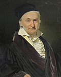
[[File:Carl Friedrich Gauss 1840 by Jensen.jpg|thumb|left|[[Carl Friedrich Gauss]] made major contributions to probabilistic methods leading to statistics.]] | |||
The mathematical foundations of statistics developed from discussions concerning [[Game of chance|games of chance]] among mathematicians such as [[Gerolamo Cardano]], [[Blaise Pascal]], [[Pierre de Fermat]], and [[Christiaan Huygens]]. Although the idea of probability was already examined in ancient and medieval law and philosophy (such as the work of [[Juan Caramuel]]), [[probability theory]] as a mathematical discipline only took shape at the very end of the 17th century, particularly in [[Jacob Bernoulli]]'s posthumous work ''{{langr|la|[[Ars Conjectandi]]}}''.<ref>{{Cite book |last=Franklin |first=James |title=The Science of Conjecture |publisher=Taylor & Francis |year=2002 |isbn=978-0-8018-7109-2 |location=Baltimore}} | |||
</ref> This was the first book where the realm of games of chance and the realm of the probable (which concerned opinion, evidence, and argument) were combined and submitted to mathematical analysis.<ref>{{multiref|{{Cite book |editor-first=I. |editor-last=Grattan-Guinness |title=Landmark Writings in Western Mathematics 1640-1940 |publisher=Elsevier |year=2005 |isbn=978-0-444-50871-3 |doi=10.1016/b978-0-444-50871-3.x5080-3 |pages=88–103}}|{{Cite book |translator-last=Sylla |translator-first=E. D. |url=https://books.google.com/books?id=-xgwSAjTh34C |title=The Art of Conjecturing, Together with Letter to a Friend on Sets in Court Tennis |last=Bernoulli |first=Jacob |publisher=Johns Hopkins University Press |year=2006 |orig-date=1713 |isbn=978-0-8018-8235-7}}}}</ref> The [[method of least squares]] was first described by [[Adrien-Marie Legendre]] in 1805, though [[Carl Friedrich Gauss]] presumably made use of it a decade earlier in 1795.<ref>{{Cite web |last=Lim |first=M. |year=2021 |title=Gauss, Least Squares, and the Missing Planet |url=https://www.actuaries.digital/2021/03/31/gauss-least-squares-and-the-missing-planet/ |access-date=2022-11-01 |website=Actuaries Digital}}</ref> | |||
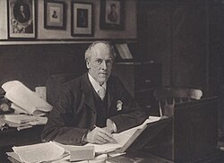
= | [[File:Karl Pearson, 1910.jpg|thumb|right|upright=1|[[Karl Pearson]], a founder of mathematical statistics]] | ||
In the 1830s-1850s, "statistical offices" and national "statistical societies" were founded in Europe and America, and in the mid-19th century, the idea arose of "organized contacts between the statisticians of different countries although informal contacts occurred earlier".<ref>J.W. Nixon, ''A history of the International Statistical Institute 1885-1960''. The Hague: International Statistical Institute, 1960, p. 5.[https://web.archive.org/web/20210905053608/https://www.isi-web.org/images/publ/J.W.Nixon.pdf]</ref> In those days, the name "statistics" referred mainly to "matters of state", and British statisticians were often called "statists".<ref>J.W. Nixon, ''A history of the International Statistical Institute 1885-1960''. The Hague: International Statistical Institute, 1960, p. 5 note 1.[https://web.archive.org/web/20210905053608/https://www.isi-web.org/images/publ/J.W.Nixon.pdf]</ref> | |||
Belgian scientist [[Adolphe Quetelet]] (1796–1874) introduced the notion of the "average man" (''l'homme moyen'') as a means of understanding complex social phenomena such as [[crime rates]], [[marriage rates]], and [[suicide rates]].<ref>{{wsPSM|Quetelet on the Science of Man|1|May 1872|first=Edward Burnett|last=Tylor|authorlink=Edward Burnett Tylor|scan=Page:Popular Science Monthly Volume 1.djvu/55}}</ref> In 1853 Quetelet organised in [[Brussels]] the [[First International Statistical Congress]] in order to unify measurement in statistical research.<ref>{{Cite book|last=Hayes|first=M.|title=Compte rendu des travaux du congrès général de statistique|year=1855|publisher=Bruxelles|hdl=2027/mdp.39015058579163}}</ref> | |||
The modern field of statistics emerged in the late 19th and early 20th century in three stages.<ref>{{Cite book |last=Walker |first=Helen Mary |author-link=Helen M. Walker |url=https://books.google.com/books?id=jYFRAAAAMAAJ |title=Studies in the history of statistical method |publisher=Arno |year=1975 |isbn=978-0405066283}}</ref> The first wave, at the turn of the century, was led by the work of [[Francis Galton]] and [[Karl Pearson]], who transformed statistics into a rigorous mathematical discipline used for analysis, not just in science, but in industry and politics as well. Galton's contributions included introducing the concepts of [[standard deviation]], [[correlation]], [[regression analysis]] and the application of these methods to the study of the variety of human characteristics—height, weight and eyelash length among others.<ref name="Galton1877">{{Cite journal |last1=Galton |first1=F. |year=1877 |title=Typical laws of heredity | url =https://archive.org/details/sim_nature-uk_1877-04-05_15_388/page/492|journal=Nature |volume=15 |issue=388 |pages=492–553 |bibcode=1877Natur..15..492. |doi=10.1038/015492a0 |doi-access=free}}</ref> Pearson developed the [[Pearson product-moment correlation coefficient]], defined as a product-moment,<ref>{{Cite journal |last1=Stigler |first1=S. M. |year=1989 |title=Francis Galton's Account of the Invention of Correlation |journal=Statistical Science |volume=4 |issue=2 |pages=73–79 |doi=10.1214/ss/1177012580 |doi-access=free}}</ref> the [[Method of moments (statistics)|method of moments]] for the fitting of distributions to samples and the [[Pearson distribution]], among many other things.<ref name="Pearson, On the criterion">{{Cite journal |last1=Pearson |first1=K. |year=1900 |title=On the Criterion that a given System of Deviations from the Probable in the Case of a Correlated System of Variables is such that it can be reasonably supposed to have arisen from Random Sampling |url=https://zenodo.org/record/1430618 |journal=Philosophical Magazine |series=Series 5 |volume=50 |issue=302 |pages=157–175 |doi=10.1080/14786440009463897}}</ref> Galton and Pearson founded ''[[Biometrika]]'' as the first journal of mathematical statistics and [[biostatistics]] (then called ''biometry''), and the latter founded the world's first university statistics department at [[University College London]].<ref>{{Cite web |title=Karl Pearson (1857–1936) |url=http://www.ucl.ac.uk/stats/department/pearson.html |url-status=dead |archive-url=https://web.archive.org/web/20080925065418/http://www.ucl.ac.uk/stats/department/pearson.html |archive-date=2008-09-25 |publisher=Department of Statistical Science, [[University College London]]}}</ref> | |||
== Methods == | The second wave of the 1910s and 20s was initiated by [[William Sealy Gosset]], and reached its culmination in the insights of [[Ronald Fisher]], who wrote the textbooks that were to define the academic discipline in universities around the world. Fisher's most important publications were his 1918 seminal paper ''[[The Correlation between Relatives on the Supposition of Mendelian Inheritance]]'' (which was the first to use the statistical term, [[variance]]), his classic 1925 work ''[[Statistical Methods for Research Workers]]'' and his 1935 ''[[The Design of Experiments]]'',<ref>{{Cite journal |last=Box |first=J. F. |date=February 1980 |title=R. A. Fisher and the Design of Experiments, 1922–1926 |journal=[[The American Statistician]] |volume=34 |issue=1 |pages=1–7 |doi=10.2307/2682986 |jstor=2682986}}</ref><ref>{{cite journal |last=Yates |first=F. |date=June 1964 |title=Sir Ronald Fisher and the Design of Experiments |journal=[[Biometrics (journal)|Biometrics]] |volume=20 |issue=2 |pages=307–321 |doi=10.2307/2528399 |jstor=2528399}}</ref><ref>{{Cite journal |last1=Stanley |first1=Julian C. |year=1966 |title=The Influence of Fisher's "The Design of Experiments" on Educational Research Thirty Years Later |journal=American Educational Research Journal |volume=3 |issue=3 |pages=223–229 |doi=10.3102/00028312003003223 |jstor=1161806 |s2cid=145725524}}</ref> where he developed rigorous [[design of experiments]] models. He originated the concepts of [[sufficiency (statistics)|sufficiency]], [[ancillary statistic]]s, [[linear discriminant analysis|Fisher's linear discriminator]] and [[Fisher information]].<ref>{{cite journal |last1=Agresti |first1=Alan |last2=Hichcock |first2=David B. |year=2005 |title=Bayesian Inference for Categorical Data Analysis |url=http://www.stat.ufl.edu/~aa/articles/agresti_hitchcock_2005.pdf |url-status=live |journal=Statistical Methods & Applications |volume=14 |issue=3 |page=298 |doi=10.1007/s10260-005-0121-y |s2cid=18896230 |archive-url=https://web.archive.org/web/20131219212926/http://www.stat.ufl.edu/~aa/articles/agresti_hitchcock_2005.pdf |archive-date=2013-12-19 |access-date=2013-12-19}}</ref> He also coined the term [[null hypothesis]] during the [[Lady tasting tea]] experiment, which "is never proved or established, but is possibly disproved, in the course of experimentation".<ref name="oed">OED quote: '''1935''' R. A. Fisher, ''[[The Design of Experiments]]'' ii. 19, "We may speak of this hypothesis as the 'null hypothesis', and the null hypothesis is never proved or established, but is possibly disproved, in the course of experimentation."</ref><ref>Fisher 1971. Chapter II: The Principles of Experimentation, Illustrated by a Psycho-physical Experiment, Section 8. The Null Hypothesis</ref> In his 1930 book ''[[The Genetical Theory of Natural Selection]]'', he applied statistics to various [[biology|biological]] concepts such as [[Fisher's principle]]<ref name="Edwards98">{{cite journal |last1=Edwards |first1=A. W. F. |year=1998 |title=Natural Selection and the Sex Ratio: Fisher's Sources |journal=American Naturalist |volume=151 |issue=6 |pages=564–569 |bibcode=1998ANat..151..564E |doi=10.1086/286141 |pmid=18811377 |s2cid=40540426}}</ref> (which [[A. W. F. Edwards]] called "probably the most celebrated argument in [[evolutionary biology]]") and [[Fisherian runaway]],<ref name="fisher15">Fisher, R. A. (1915) The evolution of sexual preference. Eugenics Review (7) 184:192</ref><ref name="fisher30">{{Cite book |last=Fisher |first=R. A. |title=The Genetical Theory of Natural Selection |title-link=The Genetical Theory of Natural Selection |publisher=Oxford University Press |year=1999 |isbn=0-19-850440-3 |orig-date=1930}}</ref><ref name="pers00">Edwards, A. W. F. (2000) Perspectives: Anecdotal, Historical and Critical Commentaries on Genetics. The Genetics Society of America (154) 1419:1426</ref><ref name="ander94">{{Cite book |last=Andersson |first=Malte |url=https://books.google.com/books?id=lNnHdvzBlTYC |title=Sexual Selection |publisher=Princeton University Press |year=1994 |isbn=0-691-00057-3}}</ref><ref name="ander06">Andersson, M. and Simmons, L. W. (2006) Sexual selection and mate choice. Trends, Ecology and Evolution (21) 296:302</ref><ref name="gayon10">Gayon, J. (2010) Sexual selection: Another Darwinian process. Comptes Rendus Biologies (333) 134:144</ref> a concept in [[sexual selection]] about a positive feedback runaway effect found in [[evolution]]. | ||
The final wave, which mainly saw the refinement and expansion of earlier developments, emerged from the collaborative work between [[Egon Pearson]] and [[Jerzy Neyman]] in the 1930s. They introduced the concepts of "[[Type I and type II errors|Type II]]" error, [[power of a test]] and [[confidence interval]]s. Jerzy Neyman in 1934 showed that stratified random sampling was in general a better method of estimation than purposive (quota) sampling.<ref>{{cite journal |last1=Neyman |first1=J. |year=1934 |title=On the two different aspects of the representative method: The method of stratified sampling and the method of purposive selection |journal=[[Journal of the Royal Statistical Society]] |volume=97 |issue=4 |pages=557–625 |doi=10.2307/2342192 |jstor=2342192}}</ref> | |||
Among the early attempts to measure national economic activity were those of [[William Petty]] in the 17th century. In the 20th century the uniform [[System of National Accounts]] was developed.<ref>[https://sk.sagepub.com/ency/edvol/businesstoday/chpt/national-accounts National Accounts]</ref> | |||
Today, statistical methods are applied in all fields that involve decision making, for making accurate inferences from a collated body of data and for making decisions in the face of uncertainty based on statistical methodology. The use of modern [[computer]]s has expedited large-scale statistical computations and has also made possible new methods that are impractical to perform manually. Statistics continues to be an area of active research, for example on the problem of how to analyze [[big data]].<ref>{{Cite web |date=2 December 2013 |title=Science in a Complex World – Big Data: Opportunity or Threat? |url=http://www.santafe.edu/news/item/sfnm-wood-big-data/ |url-status=live |archive-url=https://web.archive.org/web/20160530001750/http://www.santafe.edu/news/item/sfnm-wood-big-data/ |archive-date=2016-05-30 |access-date=2014-10-13 |work=Santa Fe Institute}}</ref> | |||
==Applications== | |||
===Applied statistics, theoretical statistics and mathematical statistics=== | |||
''Applied statistics,'' sometimes referred to as ''Statistical science,''<ref>{{Cite journal|last=Nelder|first=John A.|date=1999|title=From Statistics to Statistical Science|url=https://www.jstor.org/stable/2681191|journal=Journal of the Royal Statistical Society. Series D (The Statistician)|volume=48|issue=2|pages=257–269|doi=10.1111/1467-9884.00187|jstor=2681191|bibcode=1999JRSSD..48..257N |issn=0039-0526|access-date=2022-01-15|archive-date=2022-01-15|archive-url=https://web.archive.org/web/20220115160959/https://www.jstor.org/stable/2681191|url-status=live|url-access=subscription}}</ref> comprises descriptive statistics and the application of inferential statistics.<ref>Nikoletseas, M.M. (2014) "Statistics: Concepts and Examples." {{isbn|978-1500815684}}</ref><ref>Anderson, D.R.; Sweeney, D.J.; Williams, T.A. (1994) ''Introduction to Statistics: Concepts and Applications'', pp. 5–9. West Group. {{isbn|978-0-314-03309-3}}</ref> ''Theoretical statistics'' concerns the logical arguments underlying justification of approaches to [[statistical inference]], as well as encompassing ''mathematical statistics''. Mathematical statistics includes not only the manipulation of [[probability distribution]]s necessary for deriving results related to methods of estimation and inference, but also various aspects of [[computational statistics]] and the [[design of experiments]]. | |||
[[Statistical consultant]]s can help organizations and companies that do not have in-house expertise relevant to their particular questions. | |||
===Machine learning and data mining=== | |||
[[Machine learning]] models are statistical and probabilistic models that capture patterns in the data through use of computational algorithms. | |||
===Statistics in academia=== | |||
Statistics is applicable to a wide variety of [[academic discipline]]s, including [[Natural science|natural]] and [[social science]]s, government, and business. Business statistics applies statistical methods in [[econometrics]], [[auditing]] and production and operations, including services improvement and marketing research.<ref>{{cite web|url=https://amstat.tandfonline.com/loi/jbes|title=Journal of Business & Economic Statistics|website=Journal of Business & Economic Statistics|publisher=Taylor & Francis|access-date=16 March 2020|archive-date=27 July 2020|archive-url=https://web.archive.org/web/20200727052958/https://amstat.tandfonline.com/loi/jbes|url-status=live}}</ref> A study of two journals in tropical biology found that the 12 most frequent statistical tests are: [[analysis of variance]] (ANOVA), [[chi-squared test]], [[Student's t-test]], [[linear regression]], [[Pearson's correlation coefficient]], [[Mann-Whitney U test]], [[Kruskal-Wallis test]], [[Diversity index#Shannon index|Shannon's diversity index]], [[Tukey's range test]], [[cluster analysis]], [[Spearman's rank correlation coefficient]] and [[principal component analysis]].<ref name=":0">{{Cite journal|last=Natalia Loaiza Velásquez, María Isabel González Lutz & Julián Monge-Nájera|date=2011|title=Which statistics should tropical biologists learn?|url=https://investiga.uned.ac.cr/ecologiaurbana/wp-content/uploads/sites/30/2017/09/JMN-2011-statistics-should-learn.pdf|journal=Revista de Biología Tropical|volume=59|issue=3 |pages=983–992|pmid=22017105 |access-date=2020-04-26|archive-date=2020-10-19|archive-url=https://web.archive.org/web/20201019160957/https://investiga.uned.ac.cr/ecologiaurbana/wp-content/uploads/sites/30/2017/09/JMN-2011-statistics-should-learn.pdf|url-status=live}}</ref> | |||
A typical statistics course covers descriptive statistics, probability, binomial and [[normal distribution]]s, test of hypotheses and confidence intervals, [[linear regression]], and correlation.<ref>{{cite book|last=Pekoz|first=Erol|title=The Manager's Guide to Statistics|date=2009|publisher=Erol Pekoz|isbn=978-0979570438}}</ref> Modern fundamental statistical courses for undergraduate students focus on correct test selection, results interpretation, and use of free statistics software.<ref name=":0" /> | |||
===Statistical computing=== | |||
{{Main|Computational statistics}} | |||
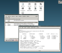
[[File:Gretl screenshot.png|thumb|upright=1.15|right|[[gretl]], an example of an [[List of open source statistical packages|open source statistical package]]]] | |||
The rapid and sustained increases in computing power starting from the second half of the 20th century have had a substantial impact on the practice of statistical science. Early statistical models were almost always from the class of [[linear model]]s, but powerful computers, coupled with suitable numerical [[algorithms]], caused an increased interest in [[Nonlinear regression|nonlinear models]] (such as [[Artificial neural network|neural networks]]) as well as the creation of new types, such as [[generalized linear model]]s and [[multilevel model]]s. | |||
Increased computing power has also led to the growing popularity of computationally intensive methods based on [[Resampling (statistics)|resampling]], such as [[permutation test]]s and the [[Bootstrapping (statistics)|bootstrap]], while techniques such as [[Gibbs sampling]] have made use of [[Bayesian model]]s more feasible. The computer revolution has implications for the future of statistics with a new emphasis on "experimental" and "empirical" statistics. A large number of both general and special purpose [[List of statistical packages|statistical software]] are now available. Examples of available software capable of complex statistical computation include programs such as [[Mathematica]], [[SAS (software)|SAS]], [[SPSS]], and [[R (programming language)|R]]. | |||
===Business statistics=== | |||
{{see also|Business mathematics#University level}} | |||
In business, "statistics" is a widely used [[Management#Nature of work|management-]] and [[decision support]] tool. It is particularly applied in [[financial management]], [[marketing management]], and [[Manufacturing process management|production]], [[operations management for services|services]] and [[operations management]].<ref>{{cite web |url=https://amstat.tandfonline.com/action/journalInformation?show=aimsScope&journalCode=ubes20 |title=Aims and scope |website=Journal of Business & Economic Statistics |publisher=Taylor & Francis |access-date=16 March 2020 |archive-date=23 June 2021 |archive-url=https://web.archive.org/web/20210623194835/https://amstat.tandfonline.com/action/journalInformation?show=aimsScope&journalCode=ubes20 |url-status=live }}</ref><ref>{{cite web |url=https://amstat.tandfonline.com/loi/jbes |title=Journal of Business & Economic Statistics |website=Journal of Business & Economic Statistics |publisher=Taylor & Francis |access-date=16 March 2020 |archive-date=27 July 2020 |archive-url=https://web.archive.org/web/20200727052958/https://amstat.tandfonline.com/loi/jbes |url-status=live }}</ref> Statistics is also heavily used in [[management accounting]] and [[auditing]]. The discipline of [[Management Science]] formalizes the use of statistics, and other mathematics, in business. ([[Econometrics]] is the application of statistical methods to [[economic data]] in order to give empirical content to [[economic theory|economic relationships]].) | |||
A typical "Business Statistics" course is intended for [[Business education#Undergraduate education|business majors]], and covers<ref>Numerous texts are available, reflecting the scope and reach of the discipline in the business world: | |||
* Sharpe, N. (2014). ''Business Statistics'', Pearson. {{ISBN|978-0134705217}} | |||
* Wegner, T. (2010). ''Applied Business Statistics: Methods and Excel-Based Applications,'' Juta Academic. {{ISBN|0702172863}} | |||
Two [[open textbook]]s are: | |||
* Holmes, L., Illowsky, B., Dean, S. (2017). [https://open.umn.edu/opentextbooks/textbooks/509 ''Introductory Business Statistics''] {{Webarchive|url=https://web.archive.org/web/20210616084059/https://open.umn.edu/opentextbooks/textbooks/509 |date=2021-06-16 }} | |||
* Nica, M. (2013). [https://open.umn.edu/opentextbooks/textbooks/384 ''Principles of Business Statistics''] {{Webarchive|url=https://web.archive.org/web/20210518151122/https://open.umn.edu/opentextbooks/textbooks/384 |date=2021-05-18 }}</ref> [[descriptive statistics]] ([[Data collection|collection]], description, analysis, and summary of data), probability (typically the [[binomial distribution|binomial]] and [[normal distribution]]s), test of hypotheses and confidence intervals, [[linear regression]], and correlation; (follow-on) courses may include [[forecasting]], [[time series]], [[decision trees]], [[multiple linear regression]], and other topics from [[business analytics]] more generally. [[Professional certification in financial services|Professional certification programs]], such as the [[Chartered Financial Analyst|CFA]], often include topics in statistics. | |||
== | == Specialized disciplines == | ||
{{main|List of fields of application of statistics}} | |||
Statistical techniques are used in a wide range of types of scientific and social research, including: [[biostatistics]], [[computational biology]], [[computational sociology]], [[network biology]], [[social science]], [[sociology]] and [[social research]]. Some fields of inquiry use applied statistics so extensively that they have [[specialized terminology]]. These disciplines include: | |||
{{Columns-list|colwidth=30em|* [[Actuarial science]] (assesses risk in the insurance and finance industries) | |||
* Applied information economics | |||
* [[Astrostatistics]] (statistical evaluation of astronomical data) | |||
* [[Biostatistics]] | |||
* [[Chemometrics]] (for analysis of data from [[chemistry]]) | |||
* [[Data mining]] (applying statistics and [[pattern recognition]] to discover knowledge from data) | |||
* [[Data science]] | |||
* [[Demography]] (statistical study of populations) | |||
* [[Econometrics]] (statistical analysis of economic data) | |||
* [[Statistical study of energy data|Energy statistics]] | |||
* [[Engineering statistics]] | |||
* [[Epidemiology]] (statistical analysis of disease) | |||
* [[Geography]] and [[geographic information system]]s, specifically in [[spatial analysis]] | |||
* [[Image processing]] | |||
* [[Jurimetrics]] ([[law]]) | |||
* [[Medical statistics]] | |||
* [[Political science]] | |||
* [[Psychological statistics]] | |||
* [[Reliability engineering]] | |||
* [[Social statistics]] | |||
* [[Statistical mechanics]]}} | |||
In addition, there are particular types of statistical analysis that have also developed their own specialised terminology and methodology: | |||
= | {{Columns-list|colwidth=30em| | ||
* [[Bootstrapping (statistics)|Bootstrap]]{{\}}[[jackknife resampling]] | |||
* [[Multivariate statistics]] | |||
* [[Statistical classification]] | |||
* [[Structured data analysis (statistics)|Structured data analysis]] | |||
* [[Structural equation modelling]] | |||
* [[Survey methodology]] | |||
* [[Survival analysis]] | |||
* Statistics in various sports, particularly [[Baseball statistics|baseball]] – known as [[sabermetrics]] – and [[Cricket statistics|cricket]] | |||
}} | |||
Statistics form a key basis tool in business and manufacturing as well. It is used to understand measurement systems variability, control processes (as in [[statistical process control]] or SPC), for summarizing data, and to make data-driven decisions. | |||
== Misuse == | |||
{{main|Misuse of statistics}} | |||
[[Misuse of statistics]] can produce subtle but serious errors in description and interpretation—subtle in the sense that even experienced professionals make such errors, and serious in the sense that they can lead to devastating decision errors. For instance, social policy, medical practice, and the reliability of structures like bridges all rely on the proper use of statistics. | |||
Even when statistical techniques are correctly applied, the results can be difficult to interpret for those lacking expertise. The [[statistical significance]] of a trend in the data—which measures the extent to which a trend could be caused by random variation in the sample—may or may not agree with an intuitive sense of its significance. The set of basic statistical skills (and skepticism) that people need to deal with information in their everyday lives properly is referred to as [[statistical literacy]]. | |||
There is a general perception that statistical knowledge is all-too-frequently intentionally [[Misuse of statistics|misused]] by finding ways to interpret only the data that are favorable to the presenter.<ref name="Huff">Huff, Darrell (1954) ''[[How to Lie with Statistics]]'', WW Norton & Company, Inc. New York. {{isbn|0-393-31072-8}}</ref> A mistrust and misunderstanding of statistics is associated with the quotation, "[[Lies, damned lies, and statistics|There are three kinds of lies: lies, damned lies, and statistics]]". Misuse of statistics can be both inadvertent and intentional, and the book ''[[How to Lie with Statistics]]'',<ref name="Huff" /> by [[Darrell Huff]], outlines a range of considerations. In an attempt to shed light on the use and misuse of statistics, reviews of statistical techniques used in particular fields are conducted (e.g. Warne, Lazo, Ramos, and Ritter (2012)).<ref>{{cite journal |last1=Warne |first1=R. Lazo |last2=Ramos |first2=T. |last3=Ritter |first3=N. |year=2012 |title=Statistical Methods Used in Gifted Education Journals, 2006–2010 |journal=Gifted Child Quarterly |volume=56 |issue=3 |pages=134–149 |doi=10.1177/0016986212444122 |s2cid=144168910}}</ref> | |||
Ways to avoid misuse of statistics include using proper diagrams and avoiding [[Bias (statistics)|bias]].<ref name="Statistics in Archaeology">{{cite book |last1=Drennan |first1=Robert D. |url=https://archive.org/details/encyclopediaarch00pear |title=Encyclopedia of Archaeology |publisher=Elsevier Inc. |year=2008 |isbn=978-0-12-373962-9 |editor-last=Pearsall |editor-first=Deborah M. |pages=[https://archive.org/details/encyclopediaarch00pear/page/n2072 2093]–2100 |chapter=Statistics in archaeology |url-access=limited}}</ref> Misuse can occur when conclusions are [[Hasty generalization|overgeneralized]] and claimed to be representative of more than they really are, often by either deliberately or unconsciously overlooking sampling bias.<ref name="Misuse of Statistics">{{cite journal |last=Cohen |first=Jerome B. |date=December 1938 |title=Misuse of Statistics |journal=Journal of the American Statistical Association |location=JSTOR |volume=33 |issue=204 |pages=657–674 |doi=10.1080/01621459.1938.10502344}}</ref> Bar graphs are arguably the easiest diagrams to use and understand, and they can be made either by hand or with simple computer programs.<ref name="Statistics in Archaeology" /> Most people do not look for bias or errors, so they are not noticed. Thus, people may often believe that something is true even if it is not well [[Sampling (statistics)|represented]].<ref name="Misuse of Statistics" /> To make data gathered from statistics believable and accurate, the sample taken must be representative of the whole.<ref name="Modern Elementary Statistics">{{cite journal |last=Freund |first=J.E. |author-link=John E. Freund |year=1988 |title=Modern Elementary Statistics |journal=Credo Reference}}</ref> According to Huff, "The dependability of a sample can be destroyed by [bias]... allow yourself some degree of skepticism."<ref>{{cite book |last=Huff |first=Darrell |title=How to Lie with Statistics |author2=Irving Geis |publisher=Norton |year=1954 |location=New York |quote=The dependability of a sample can be destroyed by [bias]... allow yourself some degree of skepticism.}}</ref> | |||
To assist in the understanding of statistics Huff proposed a series of questions to be asked in each case:<ref name="Huff" /> | |||
* Who says so? (Do they have an axe to grind?) | |||
* How do they know? (Do they have the resources to know the facts?) | |||
* What's missing? (Do they give us a complete picture?) | |||
* Did someone change the subject? (Do they offer us the right answer to the wrong problem?) | |||
* Does it make sense? (Is their conclusion logical and consistent with what we already know?) | |||
==== | ===Misinterpretation: correlation=== | ||
The | {{See also|Correlation does not imply causation}} | ||
[[File:Simple Confounding Case.svg|upright=0.9|thumb|right|The [[confounding variable]] problem: ''X'' and ''Y'' may be correlated, not because there is causal relationship between them, but because both depend on a third variable ''Z''. ''Z'' is called a confounding factor.]] | |||
The concept of [[correlation]] is particularly noteworthy for the potential confusion it can cause. Statistical analysis of a [[data set]] often reveals that two variables (properties) of the population under consideration tend to vary together, as if they were connected. For example, a study of annual income that also looks at age of death, might find that poor people tend to have shorter lives than affluent people. The two variables are said to be correlated; however, they may or may not be the cause of one another. The correlation phenomena could be caused by a third, previously unconsidered phenomenon, called a lurking variable or [[confounding variable]]. For this reason, there is no way to immediately infer the existence of a causal relationship between the two variables. | |||
== See also == | |||
{{main|Outline of statistics}} | |||
{{Portal|Mathematics}} | |||
<!-- NOTE: This is mainly for statistics-related lists. Please consider adding links to either the "Outline of statistics" or the "List of statistics articles" entries rather than here.--> | |||
{{Columns-list|colwidth=20em| | |||
* [[Abundance estimation]] | |||
* [[Glossary of probability and statistics]] | |||
* [[List of academic statistical associations]] | |||
* [[List of important publications in statistics]] | |||
* [[List of national and international statistical services]] | |||
* [[List of statistical software]] | |||
* [[List of statistics articles]] | |||
* [[List of university statistical consulting centers]] | |||
* [[Notation in probability and statistics]] | |||
* [[Statistics education]] | |||
* [[World Statistics Day]] | |||
* [[Robust statistics]] | |||
}} | |||
= | ; Foundations and major areas of statistics | ||
{{Columns-list|colwidth=22em|<!-- Foundations and major areas of statistics, closely related fields NOT already mentioned in "Specialised disciplines" section--> | |||
* [[Philosophy of statistics]] | |||
* [[Probability interpretations]] | |||
* [[Foundations of statistics]] | |||
* [[List of statisticians]] | |||
* [[Official statistics]] | |||
* [[Multivariate analysis of variance]] | |||
:<!--empty column--> | |||
:<!--empty column--> | |||
}} | |||
== References == | |||
{{reflist}} | |||
==Further reading== | |||
{{Library resources box |by=no |onlinebooks=no |others=no |about=yes |label=Statistics}} | |||
* Lydia Denworth, "A Significant Problem: Standard scientific methods are under fire. Will anything change?", ''[[Scientific American]]'', vol. 321, no. 4 (October 2019), pp. 62–67. "The use of [[p value|''p'' values]] for nearly a century [since 1925] to determine [[statistical significance]] of [[experiment]]al results has contributed to an illusion of [[certainty]] and [to] [[Replication crisis|reproducibility crises]] in many [[science|scientific fields]]. There is growing determination to reform statistical analysis... Some [researchers] suggest changing statistical methods, whereas others would do away with a threshold for defining "significant" results". (p. 63.) | |||
* {{cite book|author1=Barbara Illowsky|author2=Susan Dean|title=Introductory Statistics|url=https://openstax.org/details/introductory-statistics|year=2014|publisher=OpenStax CNX|isbn=978-1938168208}} | |||
* {{cite web|first=David W.|last=Stockburger|url=http://psychstat3.missouristate.edu/Documents/IntroBook3/sbk.htm|title=Introductory Statistics: Concepts, Models, and Applications|edition=3rd Web|website=[[Missouri State University]]|archive-url=https://web.archive.org/web/20200528093101/http://psychstat3.missouristate.edu/Documents/IntroBook3/sbk.htm|archive-date=28 May 2020}} | |||
* [https://www.openintro.org/stat/textbook.php?stat_book=os ''OpenIntro Statistics''] {{Webarchive|url=https://web.archive.org/web/20190616110442/https://www.openintro.org/stat/textbook.php?stat_book=os |date=2019-06-16 }}, 3rd edition by Diez, Barr, and Cetinkaya-Rundel | |||
* Stephen Jones, 2010. [https://web.archive.org/web/20170215092220/https://books.google.com/books?id=mywdBQAAQBAJ ''Statistics in Psychology: Explanations without Equations'']. Palgrave Macmillan. {{isbn|978-1137282392}}. | |||
* {{cite journal | last1 = Cohen | first1 = J | year = 1990 | title = Things I have learned (so far) | url = http://moityca.com.br/pdfs/Cohen_1990.pdf | archive-url = https://web.archive.org/web/20171018181831/http://moityca.com.br/pdfs/Cohen_1990.pdf | url-status = dead | archive-date = 2017-10-18 | journal = American Psychologist | volume = 45 | issue = 12 | pages = 1304–1312 | doi = 10.1037/0003-066x.45.12.1304 | s2cid = 7180431 }} | |||
* {{cite journal | last1 = Gigerenzer | first1 = G | year = 2004 | title = Mindless statistics | journal = Journal of Socio-Economics | volume = 33 | issue = 5 | pages = 587–606 | doi = 10.1016/j.socec.2004.09.033 }} | |||
* {{cite journal | last1 = Ioannidis | first1 = J.P.A. | year = 2005 | title = Why most published research findings are false | journal = PLOS Medicine | volume = 2 | issue = 4 | pages = 696–701 | doi = 10.1371/journal.pmed.0040168 | pmid = 17456002 | pmc = 1855693 | doi-access = free }} | |||
== | ==External links== | ||
{{Sister project links|Statistics}} | |||
* (Electronic Version): TIBCO Software Inc. (2020). [https://docs.tibco.com/data-science/textbook Data Science Textbook]. | |||
* [http://onlinestatbook.com/index.html ''Online Statistics Education: An Interactive Multimedia Course of Study'']. Developed by Rice University (Lead Developer), University of Houston Clear Lake, Tufts University, and National Science Foundation. | |||
* [https://web.archive.org/web/20060717201702/http://www.ats.ucla.edu/stat/ UCLA Statistical Computing Resources] (archived 17 July 2006) | |||
* [https://plato.stanford.edu/entries/statistics/ Philosophy of Statistics] from the [[Stanford Encyclopedia of Philosophy]] | |||
{{Statistics |state=expanded}} | |||
{{Areas of mathematics |collapsed}} | |||
{{Glossaries of science and engineering}} | |||
{{Authority control}} | |||
[[Category:Statistics| ]]<!--space-indexed (i.e. lead/home/eponymous) category first--> | |||
[[Category:Arab inventions]] | |||
[[Category:Data]] | |||
[[Category:Formal sciences]] | |||
[[Category:Information]] | |||
[[Category:Mathematical and quantitative methods (economics)]] | |||
[[Category: | [[Category:Research methods]] | ||
Latest revision as of 06:29, 16 March 2026


Template:StatsTopicTOC Template:Math topics TOC Statistics (from German: Statistik, orig. "description of a state, a country"[1]) is the discipline that concerns the collection, organization, analysis, interpretation, and presentation of data.[2] In applying statistics to a scientific, industrial, or social problem, it is conventional to begin with a statistical population or a statistical model to be studied. Populations can be diverse groups of people or objects such as "all people living in a country" or "every atom composing a crystal". Statistics deals with every aspect of data, including the planning of data collection in terms of the design of surveys and experiments.[3] Statistics is deeply related to subjects like physics, chemistry, geography, geopolitics, and especially mathematics.
When census data (comprising every member of the target population) cannot be collected, statisticians collect data by developing specific experiment designs and survey samples. Representative sampling assures that inferences and conclusions can reasonably extend from the sample to the population as a whole. An experimental study involves taking measurements of the system under study, manipulating the system, and then taking additional measurements using the same procedure to determine if the manipulation has modified the values of the measurements. In contrast, an observational study does not involve experimental manipulation.
Two main statistical methods are used in data analysis: descriptive statistics, which summarize data from a sample using indexes such as the mean or standard deviation, and inferential statistics, which draw conclusions from data that are subject to random variation (e.g., observational errors, sampling variation).[4] Descriptive statistics are most often concerned with two sets of properties of a distribution (sample or population): central tendency (or location) seeks to characterize the distribution's central or typical value, while dispersion (or variability) characterizes the extent to which members of the distribution depart from its center and each other. Inferences made using mathematical statistics employ the framework of probability theory, which deals with the analysis of random phenomena.
A standard statistical procedure involves the collection of data leading to a test of the relationship between two statistical data sets, or a data set and synthetic data drawn from an idealized model. A hypothesis is proposed for the statistical relationship between the two data sets, an alternative to an idealized null hypothesis of no relationship between two data sets. Rejecting or disproving the null hypothesis is done using statistical tests that quantify the sense in which the null can be proven false, given the data that are used in the test. Working from a null hypothesis, two basic forms of error are recognized: Type I errors (null hypothesis is rejected when it is in fact true, giving a "false positive") and Type II errors (null hypothesis fails to be rejected when it is in fact false, giving a "false negative"). Multiple problems have come to be associated with this framework, ranging from obtaining a sufficient sample size to specifying an adequate null hypothesis.[4]
Statistical measurement processes are also prone to error with regard to the data they generate. Many of these errors are classified as random (noise) or systematic (bias), but other types of errors (e.g., blunder, such as when an analyst reports incorrect units) can also occur. The presence of missing data or censoring may result in biased estimates, and specific techniques have been developed to address these problems.
Introduction[edit | edit source]
"Statistics is both the science of uncertainty and the technology of extracting information from data." - featured in the International Encyclopedia of Statistical Science.[5]
Statistics is the discipline that deals with data, facts and figures with which meaningful information is inferred. Data may represent a numerical value, in form of quantitative data, or a label, as with qualitative data. Data may be collected, presented and summarised, in one of two methods called descriptive statistics. Two elementary summaries of data, singularly called a statistic, are the mean and dispersion. Whereas inferential statistics interprets data from a population sample to induce statements and predictions about a population.[6][7][5]
Statistics is regarded as a body of science[8] or a branch of mathematics.[9] It is based on probability, a branch of mathematics that studies random events. Statistics is considered the science of uncertainty. This arises from the ways to cope with measurement and sampling error as well as dealing with uncertanties in modelling. Although probability and statistics were once paired together as a single subject, they are conceptually distinct from one another. The former is based on deducing answers to specific situations from a general theory of probability, meanwhile statistics induces statements about a population based on a data set. Statistics serves to bridge the gap between probability and applied mathematical fields.[10][5][11]
Some consider statistics to be a distinct mathematical science rather than a branch of mathematics. While many scientific investigations make use of data, statistics is generally concerned with the use of data in the context of uncertainty and decision-making in the face of uncertainty.[12][13] Statistics is indexed at 62, a subclass of probability theory and stochastic processes, in the Mathematics Subject Classification.[14] Mathematical statistics is covered in the range 276-280 of subclass QA (science > mathematics) in the Library of Congress Classification.[15]
The word statistics ultimately comes from the Latin word Status, meaning "situation" or "condition" in society, which in late Latin adopted the meaning "state". Derived from this, political scientist Gottfried Achenwall, coined the German word statistik (a summary of how things stand). In 1770, the term entered the English language through German and referred to the study of political arrangements. The term gained its modern meaning in the 1790s in John Sinclair's works.[16][17] In modern German, the term statistik is synonymous with mathematical statistics. The term statistic, in singular form, is used to describe a function that returns its value of the same name.[18]
Statistical data[edit | edit source]
Data collection[edit | edit source]
Sampling[edit | edit source]
When full census data cannot be collected, statisticians collect sample data by developing specific experiment designs and survey samples. Statistics itself also provides tools for prediction and forecasting through statistical models.
To use a sample as a guide to an entire population, it is important that it truly represents the overall population. Representative sampling ensures that inferences and conclusions can safely be extended from the sample to the population as a whole. A major problem lies in determining the extent to which the chosen sample is actually representative. Statistics offers methods to estimate and correct for any bias in the sample and data collection procedures. There are also methods of experimental design that can lessen these issues at the outset of a study, strengthening its ability to discern truths about the population.
Sampling theory is part of the mathematical discipline of probability theory. Probability is used in mathematical statistics to study the sampling distributions of sample statistics and, more generally, the properties of statistical procedures. The use of any statistical method is valid only when the system or population under consideration satisfies the assumptions of the method. The difference in point of view between classic probability theory and sampling theory is, roughly, that probability theory starts with the given parameters of a total population to deduce probabilities that pertain to samples. Statistical inference, however, moves in the opposite direction—inductively inferring from samples to the parameters of a larger or total population.
Experimental and observational studies[edit | edit source]
A common goal for a statistical research project is to investigate causality, and in particular to draw a conclusion on the effect of changes in the values of predictors or independent variables on dependent variables. There are two major types of causal statistical studies: experimental studies and observational studies. In both types of studies, the effect of differences of an independent variable (or variables) on the behavior of the dependent variable are observed. The difference between the two types lies in how the study is actually conducted. Each can be very effective. An experimental study involves taking measurements of the system under study, manipulating the system, and then taking additional measurements with different levels using the same procedure to determine if the manipulation has modified the values of the measurements. In contrast, an observational study does not involve experimental manipulation. Instead, data are gathered and correlations between predictors and response are investigated. While the tools of data analysis work best on data from randomized studies, they are also applied to other kinds of data—like natural experiments and observational studies[19]—for which a statistician would use a modified, more structured estimation method (e.g., difference in differences estimation and instrumental variables, among many others) that produce consistent estimators.
Experiments[edit | edit source]
The basic steps of a statistical experiment are:
- Planning the research, including finding the number of replicates of the study, using the following information: preliminary estimates regarding the size of treatment effects, alternative hypotheses, and the estimated experimental variability. Consideration of the selection of experimental subjects and the ethics of research is necessary. Statisticians recommend that experiments compare (at least) one new treatment with a standard treatment or control, to allow an unbiased estimate of the difference in treatment effects.
- Design of experiments, using blocking to reduce the influence of confounding variables, and randomized assignment of treatments to subjects to allow unbiased estimates of treatment effects and experimental error. At this stage, the experimenters and statisticians write the experimental protocol that will guide the performance of the experiment and which specifies the primary analysis of the experimental data.
- Performing the experiment following the experimental protocol and analyzing the data following the experimental protocol.
- Further examining the data set in secondary analyses, to suggest new hypotheses for future study.
- Documenting and presenting the results of the study.
Experiments on human behavior have special concerns. The famous Hawthorne study examined changes to the working environment at the Hawthorne plant of the Western Electric Company. The researchers were interested in determining whether increased illumination would increase the productivity of the assembly line workers. The researchers first measured the productivity in the plant, then modified the illumination in an area of the plant and checked if the changes in illumination affected productivity. It turned out that productivity indeed improved (under the experimental conditions). However, the study is heavily criticized today for errors in experimental procedures, specifically for the lack of a control group and blindness. The Hawthorne effect refers to finding that an outcome (in this case, worker productivity) changed due to observation itself. Those in the Hawthorne study became more productive not because the lighting was changed but because they were being observed.[20]
Observational study[edit | edit source]
An example of an observational study is one that explores the association between smoking and lung cancer. This type of study typically uses a survey to collect observations about the area of interest and then performs statistical analysis. In this case, the researchers would collect observations of both smokers and non-smokers, perhaps through a cohort study, and then look for the number of cases of lung cancer in each group.[21] A case-control study is another type of observational study in which people with and without the outcome of interest (e.g. lung cancer) are invited to participate and their exposure histories are collected.
Types of data[edit | edit source]
Various attempts have been made to produce a taxonomy of levels of measurement. The psychophysicist Stanley Smith Stevens defined nominal, ordinal, interval, and ratio scales. Nominal measurements do not have meaningful rank order among values, and permit any one-to-one (injective) transformation. Ordinal measurements have imprecise differences between consecutive values, but have a meaningful order to those values, and permit any order-preserving transformation. Interval measurements have meaningful distances between measurements defined, but the zero value is arbitrary (as in the case with longitude and temperature measurements in Celsius or Fahrenheit), and permit any linear transformation. Ratio measurements have both a meaningful zero value and the distances between different measurements defined, and permit any rescaling transformation.
Because variables conforming only to nominal or ordinal measurements cannot be reasonably measured numerically, sometimes they are grouped together as categorical variables, whereas ratio and interval measurements are grouped together as quantitative variables, which can be either discrete or continuous, due to their numerical nature. Such distinctions can often be loosely correlated with data type in computer science, in that dichotomous categorical variables may be represented with the Boolean data type, polytomous categorical variables with arbitrarily assigned integers in the integral data type, and continuous variables with the real data type involving floating-point arithmetic. But the mapping of computer science data types to statistical data types depends on which categorization of the latter is being implemented.
Other categorizations have been proposed. For example, Mosteller and Tukey (1977)[22] distinguished grades, ranks, counted fractions, counts, amounts, and balances. Nelder (1990)[23] described continuous counts, continuous ratios, count ratios, and categorical modes of data. (See also: Chrisman (1998),[24] van den Berg (1991).[25])
The issue of whether it is appropriate to apply different kinds of statistical methods to data obtained from different kinds of measurement procedures is complicated by issues concerning the transformation of variables and the precise interpretation of research questions. "The relationship between the data and what they describe merely reflects the fact that certain kinds of statistical statements may have truth values that are not invariant under some transformations. Whether a transformation is sensible to contemplate depends on the question one is trying to answer."[26]:82
Methods[edit | edit source]
 | This section needs more citations. (December 2020) |
Descriptive statistics[edit | edit source]
A descriptive statistic (in the count noun sense) is a summary statistic that quantitatively describes or summarizes features of a collection of information,[27] while descriptive statistics in the mass noun sense is the process of using and analyzing those statistics. Descriptive statistics is distinguished from inferential statistics (or inductive statistics), in that descriptive statistics aims to summarize a sample, rather than use the data to learn about the population that the sample of data is thought to represent.[28]
Inferential statistics[edit | edit source]
Statistical inference is the process of using data analysis to deduce properties of an underlying probability distribution.[29] Inferential statistical analysis infers properties of a population, for example by testing hypotheses and deriving estimates. It is assumed that the observed data set is sampled from a larger population. Inferential statistics can be contrasted with descriptive statistics. Descriptive statistics is solely concerned with properties of the observed data, and it does not rest on the assumption that the data come from a larger population.[30]
Terminology and theory of inferential statistics[edit | edit source]
Statistics, estimators and pivotal quantities[edit | edit source]
Consider independent identically distributed (IID) random variables with a given probability distribution: standard statistical inference and estimation theory defines a random sample as the random vector given by the column vector of these IID variables.[31] The population being examined is described by a probability distribution that may have unknown parameters.
A statistic is a random variable that is a function of the random sample, but not a function of unknown parameters. The probability distribution of the statistic, though, may have unknown parameters. Consider now a function of the unknown parameter: an estimator is a statistic used to estimate such function. Commonly used estimators include sample mean, unbiased sample variance and sample covariance.
A random variable that is a function of the random sample and of the unknown parameter, but whose probability distribution does not depend on the unknown parameter is called a pivotal quantity or pivot. Widely used pivots include the z-score, the chi square statistic and Student's t-value.
Between two estimators of a given parameter, the one with lower mean squared error is said to be more efficient. Furthermore, an estimator is said to be unbiased if its expected value is equal to the true value of the unknown parameter being estimated, and asymptotically unbiased if its expected value converges at the limit to the true value of such parameter.
Other desirable properties for estimators include: UMVUE estimators that have the lowest variance for all possible values of the parameter to be estimated (this is usually an easier property to verify than efficiency) and consistent estimators which converges in probability to the true value of such parameter.
This still leaves the question of how to obtain estimators in a given situation and carry the computation, several methods have been proposed: the method of moments, the maximum likelihood method, the least squares method and the more recent method of estimating equations.
Null hypothesis and alternative hypothesis[edit | edit source]
Interpretation of statistical information can often involve the development of a null hypothesis which is usually (but not necessarily) that no relationship exists among variables or that no change occurred over time.[32][33] The alternative hypothesis is the name of the hypothesis that contradicts the null hypothesis.
The best illustration for a novice is the predicament encountered by a criminal trial. The null hypothesis, H0, asserts that the defendant is innocent, whereas the alternative hypothesis, H1, asserts that the defendant is guilty. The indictment comes because of suspicion of the guilt. The H0 (the status quo) stands in opposition to H1 and is maintained unless H1 is supported by evidence "beyond a reasonable doubt". However, "failure to reject H0" in this case does not imply innocence, but merely that the evidence was insufficient to convict. So the jury does not necessarily accept H0 but fails to reject H0. While one can not "prove" a null hypothesis, one can test how close it is to being true with a power test, which tests for type II errors.
Error[edit | edit source]
Working from a null hypothesis, two broad categories of error are recognized:
- Type I errors where the null hypothesis is falsely rejected, giving a "false positive".
- Type II errors where the null hypothesis fails to be rejected and an actual difference between populations is missed, giving a "false negative".
Standard deviation refers to the extent to which individual observations in a sample differ from a central value, such as the sample or population mean, while Standard error refers to an estimate of difference between sample mean and population mean.
A statistical error is the amount by which an observation differs from its expected value. A residual is the amount an observation differs from the value the estimator of the expected value assumes on a given sample (also called prediction).
Mean squared error is used for obtaining efficient estimators, a widely used class of estimators. Root mean square error is simply the square root of mean squared error.
.svg)
Many statistical methods seek to minimize the residual sum of squares, and these are called "methods of least squares" in contrast to Least absolute deviations. The latter gives equal weight to small and big errors, while the former gives more weight to large errors. Residual sum of squares is also differentiable, which provides a handy property for doing regression. Least squares applied to linear regression is called ordinary least squares method and least squares applied to nonlinear regression is called non-linear least squares. Also in a linear regression model the non deterministic part of the model is called error term, disturbance or more simply noise. Both linear regression and non-linear regression are addressed in polynomial least squares, which also describes the variance in a prediction of the dependent variable (y axis) as a function of the independent variable (x axis) and the deviations (errors, noise, disturbances) from the estimated (fitted) curve.
Measurement processes that generate statistical data are also subject to error. Many of these errors are classified as random (noise) or systematic (bias), but other types of errors (e.g., blunder, such as when an analyst reports incorrect units) can also be important. The presence of missing data or censoring may result in biased estimates and specific techniques have been developed to address these problems.[34]
Interval estimation[edit | edit source]

Most studies only sample part of a population, so results do not fully represent the whole population. Any estimates obtained from the sample only approximate the population value. Confidence intervals allow statisticians to express how closely the sample estimate matches the true value in the whole population. Often they are expressed as 95% confidence intervals. Formally, a 95% confidence interval for a value is a range where, if the sampling and analysis were repeated under the same conditions (yielding a different dataset), the interval would include the true (population) value in 95% of all possible cases. This does not imply that the probability that the true value is in the confidence interval is 95%. From the frequentist perspective, such a claim does not even make sense, as the true value is not a random variable. Either the true value is or is not within the given interval. However, it is true that, before any data are sampled and given a plan for how to construct the confidence interval, the probability is 95% that the yet-to-be-calculated interval will cover the true value: at this point, the limits of the interval are yet-to-be-observed random variables. One approach that does yield an interval that can be interpreted as having a given probability of containing the true value is to use a credible interval from Bayesian statistics: this approach depends on a different way of interpreting what is meant by "probability", that is as a Bayesian probability.
In principle, confidence intervals can be symmetrical or asymmetrical. An interval can be asymmetrical because it works as a lower or upper bound for a parameter (left-sided interval or right sided interval), but it can also be asymmetrical if a two-sided interval is built violating symmetry around the estimate. Sometimes the bounds of a confidence interval are reached asymptotically, and these are used to approximate the true bounds.
Significance[edit | edit source]
Statistics rarely give a simple Yes/No type answer to the question under analysis. Interpretation often comes down to the level of statistical significance applied to the numbers and often refers to the probability of a value accurately rejecting the null hypothesis (sometimes referred to as the p-value).

The standard approach[31] is to test a null hypothesis against an alternative hypothesis. A critical region is the set of values of the estimator that leads to refuting the null hypothesis. The probability of type I error is therefore the probability that the estimator belongs to the critical region given that null hypothesis is true (statistical significance) and the probability of type II error is the probability that the estimator does not belong to the critical region given that the alternative hypothesis is true. The statistical power of a test is the probability that it correctly rejects the null hypothesis when the null hypothesis is false.
Referring to statistical significance does not necessarily mean that the overall result is significant in real-world terms. For example, in a large study of a drug it may be shown that the drug has a statistically significant but very small beneficial effect, such that it is unlikely to help the patient noticeably.
Although in principle the acceptable level of statistical significance may be subject to debate, the significance level is the largest p-value that allows the test to reject the null hypothesis. This test is logically equivalent to saying that the p-value is the probability, assuming the null hypothesis is true, of observing a result at least as extreme as the test statistic. Therefore, the smaller the significance level, the lower the probability of committing type I error.
Some problems are usually associated with this framework (See criticism of hypothesis testing):
- A difference that is highly statistically significant can still be of no practical significance, but it is possible to properly formulate tests to account for this. One response involves going beyond reporting only the significance level to include the p-value when reporting whether a hypothesis is rejected or accepted. The p-value, however, does not indicate the size or importance of the observed effect and can also seem to exaggerate the importance of minor differences in large studies. A better and increasingly common approach is to report confidence intervals. Although these are produced from the same calculations as those of hypothesis tests or p-values, they describe both the size of the effect and the uncertainty surrounding it.
- Fallacy of the transposed conditional, aka prosecutor's fallacy: criticisms arise because the hypothesis testing approach forces one hypothesis (the null hypothesis) to be favored, since what is being evaluated is the probability of the observed result given the null hypothesis and not probability of the null hypothesis given the observed result. An alternative to this approach is offered by Bayesian inference, although it requires establishing a prior probability.[35]
- Rejecting the null hypothesis does not automatically prove the alternative hypothesis.
- As everything in inferential statistics it relies on sample size, and therefore under fat tails p-values may be seriously mis-computed.[clarification needed]
Examples[edit | edit source]
Some well-known statistical tests and procedures are:
Bayesian statistics[edit | edit source]
An alternative paradigm to the popular frequentist paradigm is to use Bayes' theorem to update the prior probability of the hypotheses in consideration based on the relative likelihood of the evidence gathered to obtain a posterior probability. Bayesian methods have been aided by the increase in available computing power to compute the posterior probability using numerical approximation techniques like Markov Chain Monte Carlo.
For statistically modelling purposes, Bayesian models tend to be hierarchical, for example, one could model each YouTube channel as having video views distributed as a normal distribution with channel dependent mean and variance , while modeling the channel means as themselves coming from a normal distribution representing the distribution of average video view counts per channel, and the variances as coming from another distribution.
The concept of using likelihood ratio can also be prominently seen in medical diagnostic testing.
Exploratory data analysis[edit | edit source]
Exploratory data analysis (EDA) is an approach to analyzing data sets to summarize their main characteristics, often with visual methods. A statistical model can be used or not, but primarily EDA is for seeing what the data can tell us beyond the formal modeling or hypothesis testing task.
Mathematical statistics[edit | edit source]
Mathematical statistics is the application of mathematics to statistics. Mathematical techniques used for this include mathematical analysis, linear algebra, stochastic analysis, differential equations, and measure-theoretic probability theory.[1][7] All statistical analyses make use of at least some mathematics, and mathematical statistics can therefore be regarded as a fundamental component of general statistics.[8]
History[edit | edit source]

Formal discussions on inference date back to the mathematicians and cryptographers of the Islamic Golden Age between the 8th and 13th centuries. Al-Khalil (717–786) wrote the Book of Cryptographic Messages, which contains one of the first uses of permutations and combinations, to list all possible Arabic words with and without vowels.[36] Al-Kindi's Manuscript on Deciphering Cryptographic Messages gave a detailed description of how to use frequency analysis to decipher encrypted messages, providing an early example of statistical inference for decoding. Ibn Adlan (1187–1268) later made an important contribution on the use of sample size in frequency analysis.[36]
Although the term statistic was introduced by the Italian scholar Girolamo Ghilini in 1589 with reference to a collection of facts and information about a state, it was the German Gottfried Achenwall in 1749 who started using the term as a collection of quantitative information, in the modern use for this science.[37][38] The earliest writing containing statistics in Europe dates back to 1663, with the publication of Natural and Political Observations upon the Bills of Mortality by John Graunt.[39]
Early applications of statistical thinking revolved around the needs of states to base policy on demographic and economic data, hence its stat- etymology. The scope of the discipline of statistics broadened in the early 19th century to include the collection and analysis of data in general. Today, statistics is widely employed in government, business, and natural and social sciences.

The mathematical foundations of statistics developed from discussions concerning games of chance among mathematicians such as Gerolamo Cardano, Blaise Pascal, Pierre de Fermat, and Christiaan Huygens. Although the idea of probability was already examined in ancient and medieval law and philosophy (such as the work of Juan Caramuel), probability theory as a mathematical discipline only took shape at the very end of the 17th century, particularly in Jacob Bernoulli's posthumous work Template:Langr.[40] This was the first book where the realm of games of chance and the realm of the probable (which concerned opinion, evidence, and argument) were combined and submitted to mathematical analysis.[41] The method of least squares was first described by Adrien-Marie Legendre in 1805, though Carl Friedrich Gauss presumably made use of it a decade earlier in 1795.[42]

In the 1830s-1850s, "statistical offices" and national "statistical societies" were founded in Europe and America, and in the mid-19th century, the idea arose of "organized contacts between the statisticians of different countries although informal contacts occurred earlier".[43] In those days, the name "statistics" referred mainly to "matters of state", and British statisticians were often called "statists".[44]
Belgian scientist Adolphe Quetelet (1796–1874) introduced the notion of the "average man" (l'homme moyen) as a means of understanding complex social phenomena such as crime rates, marriage rates, and suicide rates.[45] In 1853 Quetelet organised in Brussels the First International Statistical Congress in order to unify measurement in statistical research.[46]
The modern field of statistics emerged in the late 19th and early 20th century in three stages.[47] The first wave, at the turn of the century, was led by the work of Francis Galton and Karl Pearson, who transformed statistics into a rigorous mathematical discipline used for analysis, not just in science, but in industry and politics as well. Galton's contributions included introducing the concepts of standard deviation, correlation, regression analysis and the application of these methods to the study of the variety of human characteristics—height, weight and eyelash length among others.[48] Pearson developed the Pearson product-moment correlation coefficient, defined as a product-moment,[49] the method of moments for the fitting of distributions to samples and the Pearson distribution, among many other things.[50] Galton and Pearson founded Biometrika as the first journal of mathematical statistics and biostatistics (then called biometry), and the latter founded the world's first university statistics department at University College London.[51]
The second wave of the 1910s and 20s was initiated by William Sealy Gosset, and reached its culmination in the insights of Ronald Fisher, who wrote the textbooks that were to define the academic discipline in universities around the world. Fisher's most important publications were his 1918 seminal paper The Correlation between Relatives on the Supposition of Mendelian Inheritance (which was the first to use the statistical term, variance), his classic 1925 work Statistical Methods for Research Workers and his 1935 The Design of Experiments,[52][53][54] where he developed rigorous design of experiments models. He originated the concepts of sufficiency, ancillary statistics, Fisher's linear discriminator and Fisher information.[55] He also coined the term null hypothesis during the Lady tasting tea experiment, which "is never proved or established, but is possibly disproved, in the course of experimentation".[56][57] In his 1930 book The Genetical Theory of Natural Selection, he applied statistics to various biological concepts such as Fisher's principle[58] (which A. W. F. Edwards called "probably the most celebrated argument in evolutionary biology") and Fisherian runaway,[59][60][61][62][63][64] a concept in sexual selection about a positive feedback runaway effect found in evolution.
The final wave, which mainly saw the refinement and expansion of earlier developments, emerged from the collaborative work between Egon Pearson and Jerzy Neyman in the 1930s. They introduced the concepts of "Type II" error, power of a test and confidence intervals. Jerzy Neyman in 1934 showed that stratified random sampling was in general a better method of estimation than purposive (quota) sampling.[65]
Among the early attempts to measure national economic activity were those of William Petty in the 17th century. In the 20th century the uniform System of National Accounts was developed.[66]
Today, statistical methods are applied in all fields that involve decision making, for making accurate inferences from a collated body of data and for making decisions in the face of uncertainty based on statistical methodology. The use of modern computers has expedited large-scale statistical computations and has also made possible new methods that are impractical to perform manually. Statistics continues to be an area of active research, for example on the problem of how to analyze big data.[67]
Applications[edit | edit source]
Applied statistics, theoretical statistics and mathematical statistics[edit | edit source]
Applied statistics, sometimes referred to as Statistical science,[68] comprises descriptive statistics and the application of inferential statistics.[69][70] Theoretical statistics concerns the logical arguments underlying justification of approaches to statistical inference, as well as encompassing mathematical statistics. Mathematical statistics includes not only the manipulation of probability distributions necessary for deriving results related to methods of estimation and inference, but also various aspects of computational statistics and the design of experiments.
Statistical consultants can help organizations and companies that do not have in-house expertise relevant to their particular questions.
Machine learning and data mining[edit | edit source]
Machine learning models are statistical and probabilistic models that capture patterns in the data through use of computational algorithms.
Statistics in academia[edit | edit source]
Statistics is applicable to a wide variety of academic disciplines, including natural and social sciences, government, and business. Business statistics applies statistical methods in econometrics, auditing and production and operations, including services improvement and marketing research.[71] A study of two journals in tropical biology found that the 12 most frequent statistical tests are: analysis of variance (ANOVA), chi-squared test, Student's t-test, linear regression, Pearson's correlation coefficient, Mann-Whitney U test, Kruskal-Wallis test, Shannon's diversity index, Tukey's range test, cluster analysis, Spearman's rank correlation coefficient and principal component analysis.[72]
A typical statistics course covers descriptive statistics, probability, binomial and normal distributions, test of hypotheses and confidence intervals, linear regression, and correlation.[73] Modern fundamental statistical courses for undergraduate students focus on correct test selection, results interpretation, and use of free statistics software.[72]
Statistical computing[edit | edit source]

The rapid and sustained increases in computing power starting from the second half of the 20th century have had a substantial impact on the practice of statistical science. Early statistical models were almost always from the class of linear models, but powerful computers, coupled with suitable numerical algorithms, caused an increased interest in nonlinear models (such as neural networks) as well as the creation of new types, such as generalized linear models and multilevel models.
Increased computing power has also led to the growing popularity of computationally intensive methods based on resampling, such as permutation tests and the bootstrap, while techniques such as Gibbs sampling have made use of Bayesian models more feasible. The computer revolution has implications for the future of statistics with a new emphasis on "experimental" and "empirical" statistics. A large number of both general and special purpose statistical software are now available. Examples of available software capable of complex statistical computation include programs such as Mathematica, SAS, SPSS, and R.
Business statistics[edit | edit source]
In business, "statistics" is a widely used management- and decision support tool. It is particularly applied in financial management, marketing management, and production, services and operations management.[74][75] Statistics is also heavily used in management accounting and auditing. The discipline of Management Science formalizes the use of statistics, and other mathematics, in business. (Econometrics is the application of statistical methods to economic data in order to give empirical content to economic relationships.)
A typical "Business Statistics" course is intended for business majors, and covers[76] descriptive statistics (collection, description, analysis, and summary of data), probability (typically the binomial and normal distributions), test of hypotheses and confidence intervals, linear regression, and correlation; (follow-on) courses may include forecasting, time series, decision trees, multiple linear regression, and other topics from business analytics more generally. Professional certification programs, such as the CFA, often include topics in statistics.
Specialized disciplines[edit | edit source]
Statistical techniques are used in a wide range of types of scientific and social research, including: biostatistics, computational biology, computational sociology, network biology, social science, sociology and social research. Some fields of inquiry use applied statistics so extensively that they have specialized terminology. These disciplines include:
- Actuarial science (assesses risk in the insurance and finance industries)
- Applied information economics
- Astrostatistics (statistical evaluation of astronomical data)
- Biostatistics
- Chemometrics (for analysis of data from chemistry)
- Data mining (applying statistics and pattern recognition to discover knowledge from data)
- Data science
- Demography (statistical study of populations)
- Econometrics (statistical analysis of economic data)
- Energy statistics
- Engineering statistics
- Epidemiology (statistical analysis of disease)
- Geography and geographic information systems, specifically in spatial analysis
- Image processing
- Jurimetrics (law)
- Medical statistics
- Political science
- Psychological statistics
- Reliability engineering
- Social statistics
- Statistical mechanics
In addition, there are particular types of statistical analysis that have also developed their own specialised terminology and methodology:
- Bootstrap / jackknife resampling
- Multivariate statistics
- Statistical classification
- Structured data analysis
- Structural equation modelling
- Survey methodology
- Survival analysis
- Statistics in various sports, particularly baseball – known as sabermetrics – and cricket
Statistics form a key basis tool in business and manufacturing as well. It is used to understand measurement systems variability, control processes (as in statistical process control or SPC), for summarizing data, and to make data-driven decisions.
Misuse[edit | edit source]
Misuse of statistics can produce subtle but serious errors in description and interpretation—subtle in the sense that even experienced professionals make such errors, and serious in the sense that they can lead to devastating decision errors. For instance, social policy, medical practice, and the reliability of structures like bridges all rely on the proper use of statistics.
Even when statistical techniques are correctly applied, the results can be difficult to interpret for those lacking expertise. The statistical significance of a trend in the data—which measures the extent to which a trend could be caused by random variation in the sample—may or may not agree with an intuitive sense of its significance. The set of basic statistical skills (and skepticism) that people need to deal with information in their everyday lives properly is referred to as statistical literacy.
There is a general perception that statistical knowledge is all-too-frequently intentionally misused by finding ways to interpret only the data that are favorable to the presenter.[77] A mistrust and misunderstanding of statistics is associated with the quotation, "There are three kinds of lies: lies, damned lies, and statistics". Misuse of statistics can be both inadvertent and intentional, and the book How to Lie with Statistics,[77] by Darrell Huff, outlines a range of considerations. In an attempt to shed light on the use and misuse of statistics, reviews of statistical techniques used in particular fields are conducted (e.g. Warne, Lazo, Ramos, and Ritter (2012)).[78]
Ways to avoid misuse of statistics include using proper diagrams and avoiding bias.[79] Misuse can occur when conclusions are overgeneralized and claimed to be representative of more than they really are, often by either deliberately or unconsciously overlooking sampling bias.[80] Bar graphs are arguably the easiest diagrams to use and understand, and they can be made either by hand or with simple computer programs.[79] Most people do not look for bias or errors, so they are not noticed. Thus, people may often believe that something is true even if it is not well represented.[80] To make data gathered from statistics believable and accurate, the sample taken must be representative of the whole.[81] According to Huff, "The dependability of a sample can be destroyed by [bias]... allow yourself some degree of skepticism."[82]
To assist in the understanding of statistics Huff proposed a series of questions to be asked in each case:[77]
- Who says so? (Do they have an axe to grind?)
- How do they know? (Do they have the resources to know the facts?)
- What's missing? (Do they give us a complete picture?)
- Did someone change the subject? (Do they offer us the right answer to the wrong problem?)
- Does it make sense? (Is their conclusion logical and consistent with what we already know?)
Misinterpretation: correlation[edit | edit source]

The concept of correlation is particularly noteworthy for the potential confusion it can cause. Statistical analysis of a data set often reveals that two variables (properties) of the population under consideration tend to vary together, as if they were connected. For example, a study of annual income that also looks at age of death, might find that poor people tend to have shorter lives than affluent people. The two variables are said to be correlated; however, they may or may not be the cause of one another. The correlation phenomena could be caused by a third, previously unconsidered phenomenon, called a lurking variable or confounding variable. For this reason, there is no way to immediately infer the existence of a causal relationship between the two variables.
See also[edit | edit source]
- Abundance estimation
- Glossary of probability and statistics
- List of academic statistical associations
- List of important publications in statistics
- List of national and international statistical services
- List of statistical software
- List of statistics articles
- List of university statistical consulting centers
- Notation in probability and statistics
- Statistics education
- World Statistics Day
- Robust statistics
- Foundations and major areas of statistics
- Philosophy of statistics
- Probability interpretations
- Foundations of statistics
- List of statisticians
- Official statistics
- Multivariate analysis of variance
References[edit | edit source]
- ↑ 1.0 1.1 Template:Multiref
- ↑ Template:Multiref
- ↑ Dodge, Yadolah (2003). The Oxford Dictionary of Statistical Terms. Oxford University Press. ISBN 0-19-920613-9.
- ↑ 4.0 4.1 Lund Research Ltd. "Descriptive and Inferential Statistics". statistics.laerd.com. Archived from the original on 2020-10-26. Retrieved 2014-03-23.
- ↑ 5.0 5.1 5.2 Hand, David (2010). "Statistics: An Overview". In Lovric, Miodrag (ed.). International Encyclopedia of Statistical Science. Springer. pp. 1504–1509. ISBN 978-3-642-04898-2.
- ↑ Tanton, James (2005). "Statistics". Encyclopedia of Mathematics. Facts On File. pp. 478–484. ISBN 0-8160-5124-0.
- ↑ 7.0 7.1 "Statistics | Definition, Types, & Importance | Britannica". www.britannica.com. 2024-12-06. Retrieved 2024-12-30.
- ↑ 8.0 8.1 Moses, Lincoln E. (1986) Think and Explain with Statistics, Addison-Wesley, ISBN 978-0-201-15619-5. pp. 1–3
- ↑ Hays, William Lee, (1973) Statistics for the Social Sciences, Holt, Rinehart and Winston, p. xii, ISBN 978-0-03-077945-9
- ↑ Williams, David (2001). "Preface". Weighing the Odds: A Course in Probability and Statistics. Cambridge University Press. pp. xi–xvii. ISBN 9780521006187.
- ↑ Rudas, Tamas (2010). "Probability Theory: An Outline". In Lovric, Miodrag (ed.). International Encyclopedia of Statistical Science. Springer. pp. 1123–1126. ISBN 978-3-642-04898-2.
- ↑ Moore, David (1992). "Teaching Statistics as a Respectable Subject". In F. Gordon; S. Gordon (eds.). Statistics for the Twenty-First Century. Washington, DC: The Mathematical Association of America. pp. 14–25. ISBN 978-0-88385-078-7.
- ↑ Chance, Beth L.; Rossman, Allan J. (2005). "Preface" (PDF). Investigating Statistical Concepts, Applications, and Methods. Duxbury Press. ISBN 978-0-495-05064-3. Archived (PDF) from the original on 2020-11-22. Retrieved 2009-12-06.
- ↑ "Classification Search Result - zbMATH Open". zbmath.org. Retrieved 2024-12-30.
- ↑ Higham, Nicholas J. (1998). "Aids and Resources for Writing and Research". Handbook of Writing for the Mathematical Sciences. Society for Industrial and Applied Mathematics. p. 214. ISBN 0-89871-420-6.
- ↑ Sheynin, Oscar (2010). "Statistics, History of". In Lovric, Miodrag (ed.). International Encyclopedia of Statistical Science. Springer. pp. 1493–1504. ISBN 978-3-642-04898-2.
- ↑ Hoad, T. F., ed. (1996). The Concise Oxford Dictionary of English Etymology. Oxford University Press. p. 460. ISBN 0-19-283098-8.
- ↑ "Statistik". www.spektrum.de (in Deutsch). Retrieved 2024-12-30.
- ↑ Freedman, D.A. (2005) Statistical Models: Theory and Practice, Cambridge University Press. ISBN 978-0-521-67105-7
- ↑ McCarney R, Warner J, Iliffe S, van Haselen R, Griffin M, Fisher P (2007). "The Hawthorne Effect: a randomised, controlled trial". BMC Med Res Methodol. 7 (1) 30. doi:10.1186/1471-2288-7-30. PMC 1936999. PMID 17608932.
- ↑ Rothman, Kenneth J; Greenland, Sander; Lash, Timothy, eds. (2008). "7". Modern Epidemiology (3rd ed.). Lippincott Williams & Wilkins. p. 100. ISBN 978-0781755641.
- ↑ Mosteller, F.; Tukey, J.W (1977). Data analysis and regression. Boston: Addison-Wesley.
- ↑ Nelder, J.A. (1990). The knowledge needed to computerise the analysis and interpretation of statistical information. In Expert systems and artificial intelligence: the need for information about data. Library Association Report, London, March, 23–27.
- ↑ Chrisman, Nicholas R (1998). "Rethinking Levels of Measurement for Cartography". Cartography and Geographic Information Science. 25 (4): 231–242. Bibcode:1998CGISy..25..231C. doi:10.1559/152304098782383043.
- ↑ van den Berg, G. (1991). Choosing an analysis method. Leiden: DSWO Press
- ↑ Hand, D.J. (2004). Measurement theory and practice: The world through quantification. London: Arnold.
- ↑ Mann, Prem S. (1995). Introductory Statistics (2nd ed.). Wiley. ISBN 0-471-31009-3.
- ↑ "Descriptive Statistics | Research Connections". www.researchconnections.org. Retrieved 2023-01-10.
- ↑ Upton, G., Cook, I. (2008) Oxford Dictionary of Statistics, OUP. ISBN 978-0-19-954145-4.
- ↑ "Basic Inferential Statistics - Purdue OWL - Purdue University". owl.purdue.edu. Retrieved 2023-01-10.
- ↑ 31.0 31.1 Piazza Elio, Probabilità e Statistica, Esculapio 2007
- ↑ Everitt, Brian (1998). The Cambridge Dictionary of Statistics. Cambridge, UK New York: Cambridge University Press. ISBN 0521593468.
- ↑ "Cohen (1994) The Earth Is Round (p < .05)". YourStatsGuru.com. Archived from the original on 2015-09-05. Retrieved 2015-07-20.
- ↑ Rubin, Donald B.; Little, Roderick J.A., Statistical analysis with missing data, New York: Wiley 2002
- ↑ Ioannidis, J.P.A. (2005). "Why Most Published Research Findings Are False". PLOS Medicine. 2 (8): e124. doi:10.1371/journal.pmed.0020124. PMC 1182327. PMID 16060722.
- ↑ 36.0 36.1 Broemeling, Lyle D. (1 November 2011). "An Account of Early Statistical Inference in Arab Cryptology". The American Statistician. 65 (4): 255–257. doi:10.1198/tas.2011.10191. S2CID 123537702.
- ↑ Ostasiewicz, Walenty (2014). "The emergence of statistical science". Śląski Przegląd Statystyczny. 12 (18): 76–77. doi:10.15611/sps.2014.12.04.
- ↑ Bruneau, Quentin (2022). States and the Masters of Capital: Sovereign Lending, Old and New. Columbia University Press. ISBN 978-0231555647.
- ↑ Willcox, Walter (1938) "The Founder of Statistics". Review of the International Statistical Institute 5(4): 321–328. JSTOR 1400906
- ↑ Franklin, James (2002). The Science of Conjecture. Baltimore: Taylor & Francis. ISBN 978-0-8018-7109-2.
- ↑ Template:Multiref
- ↑ Lim, M. (2021). "Gauss, Least Squares, and the Missing Planet". Actuaries Digital. Retrieved 2022-11-01.
- ↑ J.W. Nixon, A history of the International Statistical Institute 1885-1960. The Hague: International Statistical Institute, 1960, p. 5.[1]
- ↑ J.W. Nixon, A history of the International Statistical Institute 1885-1960. The Hague: International Statistical Institute, 1960, p. 5 note 1.[2]
- ↑ Template:WsPSM
- ↑ Hayes, M. (1855). Compte rendu des travaux du congrès général de statistique. Bruxelles. hdl:2027/mdp.39015058579163.
- ↑ Walker, Helen Mary (1975). Studies in the history of statistical method. Arno. ISBN 978-0405066283.
- ↑ Galton, F. (1877). "Typical laws of heredity". Nature. 15 (388): 492–553. Bibcode:1877Natur..15..492.. doi:10.1038/015492a0.
- ↑ Stigler, S. M. (1989). "Francis Galton's Account of the Invention of Correlation". Statistical Science. 4 (2): 73–79. doi:10.1214/ss/1177012580.
- ↑ Pearson, K. (1900). "On the Criterion that a given System of Deviations from the Probable in the Case of a Correlated System of Variables is such that it can be reasonably supposed to have arisen from Random Sampling". Philosophical Magazine. Series 5. 50 (302): 157–175. doi:10.1080/14786440009463897.
- ↑ "Karl Pearson (1857–1936)". Department of Statistical Science, University College London. Archived from the original on 2008-09-25.
- ↑ Box, J. F. (February 1980). "R. A. Fisher and the Design of Experiments, 1922–1926". The American Statistician. 34 (1): 1–7. doi:10.2307/2682986. JSTOR 2682986.
- ↑ Yates, F. (June 1964). "Sir Ronald Fisher and the Design of Experiments". Biometrics. 20 (2): 307–321. doi:10.2307/2528399. JSTOR 2528399.
- ↑ Stanley, Julian C. (1966). "The Influence of Fisher's "The Design of Experiments" on Educational Research Thirty Years Later". American Educational Research Journal. 3 (3): 223–229. doi:10.3102/00028312003003223. JSTOR 1161806. S2CID 145725524.
- ↑ Agresti, Alan; Hichcock, David B. (2005). "Bayesian Inference for Categorical Data Analysis" (PDF). Statistical Methods & Applications. 14 (3): 298. doi:10.1007/s10260-005-0121-y. S2CID 18896230. Archived (PDF) from the original on 2013-12-19. Retrieved 2013-12-19.
- ↑ OED quote: 1935 R. A. Fisher, The Design of Experiments ii. 19, "We may speak of this hypothesis as the 'null hypothesis', and the null hypothesis is never proved or established, but is possibly disproved, in the course of experimentation."
- ↑ Fisher 1971. Chapter II: The Principles of Experimentation, Illustrated by a Psycho-physical Experiment, Section 8. The Null Hypothesis
- ↑ Edwards, A. W. F. (1998). "Natural Selection and the Sex Ratio: Fisher's Sources". American Naturalist. 151 (6): 564–569. Bibcode:1998ANat..151..564E. doi:10.1086/286141. PMID 18811377. S2CID 40540426.
- ↑ Fisher, R. A. (1915) The evolution of sexual preference. Eugenics Review (7) 184:192
- ↑ Fisher, R. A. (1999) [1930]. The Genetical Theory of Natural Selection. Oxford University Press. ISBN 0-19-850440-3.
- ↑ Edwards, A. W. F. (2000) Perspectives: Anecdotal, Historical and Critical Commentaries on Genetics. The Genetics Society of America (154) 1419:1426
- ↑ Andersson, Malte (1994). Sexual Selection. Princeton University Press. ISBN 0-691-00057-3.
- ↑ Andersson, M. and Simmons, L. W. (2006) Sexual selection and mate choice. Trends, Ecology and Evolution (21) 296:302
- ↑ Gayon, J. (2010) Sexual selection: Another Darwinian process. Comptes Rendus Biologies (333) 134:144
- ↑ Neyman, J. (1934). "On the two different aspects of the representative method: The method of stratified sampling and the method of purposive selection". Journal of the Royal Statistical Society. 97 (4): 557–625. doi:10.2307/2342192. JSTOR 2342192.
- ↑ National Accounts
- ↑ "Science in a Complex World – Big Data: Opportunity or Threat?". Santa Fe Institute. 2 December 2013. Archived from the original on 2016-05-30. Retrieved 2014-10-13.
- ↑ Nelder, John A. (1999). "From Statistics to Statistical Science". Journal of the Royal Statistical Society. Series D (The Statistician). 48 (2): 257–269. Bibcode:1999JRSSD..48..257N. doi:10.1111/1467-9884.00187. ISSN 0039-0526. JSTOR 2681191. Archived from the original on 2022-01-15. Retrieved 2022-01-15.
- ↑ Nikoletseas, M.M. (2014) "Statistics: Concepts and Examples." ISBN 978-1500815684
- ↑ Anderson, D.R.; Sweeney, D.J.; Williams, T.A. (1994) Introduction to Statistics: Concepts and Applications, pp. 5–9. West Group. ISBN 978-0-314-03309-3
- ↑ "Journal of Business & Economic Statistics". Journal of Business & Economic Statistics. Taylor & Francis. Archived from the original on 27 July 2020. Retrieved 16 March 2020.
- ↑ 72.0 72.1 Natalia Loaiza Velásquez, María Isabel González Lutz & Julián Monge-Nájera (2011). "Which statistics should tropical biologists learn?" (PDF). Revista de Biología Tropical. 59 (3): 983–992. PMID 22017105. Archived (PDF) from the original on 2020-10-19. Retrieved 2020-04-26.
- ↑ Pekoz, Erol (2009). The Manager's Guide to Statistics. Erol Pekoz. ISBN 978-0979570438.
- ↑ "Aims and scope". Journal of Business & Economic Statistics. Taylor & Francis. Archived from the original on 23 June 2021. Retrieved 16 March 2020.
- ↑ "Journal of Business & Economic Statistics". Journal of Business & Economic Statistics. Taylor & Francis. Archived from the original on 27 July 2020. Retrieved 16 March 2020.
- ↑ Numerous texts are available, reflecting the scope and reach of the discipline in the business world:
- Sharpe, N. (2014). Business Statistics, Pearson. ISBN 978-0134705217
- Wegner, T. (2010). Applied Business Statistics: Methods and Excel-Based Applications, Juta Academic. ISBN 0702172863
- Holmes, L., Illowsky, B., Dean, S. (2017). Introductory Business Statistics Archived 2021-06-16 at the Wayback Machine
- Nica, M. (2013). Principles of Business Statistics Archived 2021-05-18 at the Wayback Machine
- ↑ 77.0 77.1 77.2 Huff, Darrell (1954) How to Lie with Statistics, WW Norton & Company, Inc. New York. ISBN 0-393-31072-8
- ↑ Warne, R. Lazo; Ramos, T.; Ritter, N. (2012). "Statistical Methods Used in Gifted Education Journals, 2006–2010". Gifted Child Quarterly. 56 (3): 134–149. doi:10.1177/0016986212444122. S2CID 144168910.
- ↑ 79.0 79.1 Drennan, Robert D. (2008). "Statistics in archaeology". In Pearsall, Deborah M. (ed.). Encyclopedia of Archaeology. Elsevier Inc. pp. 2093–2100. ISBN 978-0-12-373962-9.
- ↑ 80.0 80.1 Cohen, Jerome B. (December 1938). "Misuse of Statistics". Journal of the American Statistical Association. 33 (204). JSTOR: 657–674. doi:10.1080/01621459.1938.10502344.
- ↑ Freund, J.E. (1988). "Modern Elementary Statistics". Credo Reference.
- ↑ Huff, Darrell; Irving Geis (1954). How to Lie with Statistics. New York: Norton.
The dependability of a sample can be destroyed by [bias]... allow yourself some degree of skepticism.
Further reading[edit | edit source]
| Library resources about Statistics |
- Lydia Denworth, "A Significant Problem: Standard scientific methods are under fire. Will anything change?", Scientific American, vol. 321, no. 4 (October 2019), pp. 62–67. "The use of p values for nearly a century [since 1925] to determine statistical significance of experimental results has contributed to an illusion of certainty and [to] reproducibility crises in many scientific fields. There is growing determination to reform statistical analysis... Some [researchers] suggest changing statistical methods, whereas others would do away with a threshold for defining "significant" results". (p. 63.)
- Barbara Illowsky; Susan Dean (2014). Introductory Statistics. OpenStax CNX. ISBN 978-1938168208.
- Stockburger, David W. "Introductory Statistics: Concepts, Models, and Applications". Missouri State University (3rd Web ed.). Archived from the original on 28 May 2020.
- OpenIntro Statistics Archived 2019-06-16 at the Wayback Machine, 3rd edition by Diez, Barr, and Cetinkaya-Rundel
- Stephen Jones, 2010. Statistics in Psychology: Explanations without Equations. Palgrave Macmillan. ISBN 978-1137282392.
- Cohen, J (1990). "Things I have learned (so far)" (PDF). American Psychologist. 45 (12): 1304–1312. doi:10.1037/0003-066x.45.12.1304. S2CID 7180431. Archived from the original (PDF) on 2017-10-18.
- Gigerenzer, G (2004). "Mindless statistics". Journal of Socio-Economics. 33 (5): 587–606. doi:10.1016/j.socec.2004.09.033.
- Ioannidis, J.P.A. (2005). "Why most published research findings are false". PLOS Medicine. 2 (4): 696–701. doi:10.1371/journal.pmed.0040168. PMC 1855693. PMID 17456002.
External links[edit | edit source]
- (Electronic Version): TIBCO Software Inc. (2020). Data Science Textbook.
- Online Statistics Education: An Interactive Multimedia Course of Study. Developed by Rice University (Lead Developer), University of Houston Clear Lake, Tufts University, and National Science Foundation.
- UCLA Statistical Computing Resources (archived 17 July 2006)
- Philosophy of Statistics from the Stanford Encyclopedia of Philosophy


Template:Areas of mathematics Template:Glossaries of science and engineering