Synthetic-aperture radar

For broader coverage of this topic, see Radar imaging.

This radar image acquired by the SIR-C/X-SAR radar on board the Space Shuttle Endeavour shows the Teide volcano. The city of Santa Cruz de Tenerife is visible as the purple and white area on the lower right edge of the island. Lava flows at the summit crater appear in shades of green and brown, while vegetation zones appear as areas of purple, green and yellow on the volcano's flanks.

Synthetic-aperture radar (SAR) is a form of radar that is used to create two-dimensional images or three-dimensional reconstructions of objects, such as landscapes. SAR uses the motion of the radar antenna over a target region to provide finer spatial resolution than conventional stationary beam-scanning radars. SAR is typically mounted on a moving platform, such as an aircraft or spacecraft, and has its origins in an advanced form of side looking airborne radar (SLAR). The distance the SAR device travels over a target during the period when the target scene is illuminated creates the large synthetic antenna aperture (the size of the antenna). Typically, the larger the aperture, the higher the image resolution will be, regardless of whether the aperture is physical (a large antenna) or synthetic (a moving antenna) – this allows SAR to create high-resolution images with comparatively small physical antennas. For a fixed antenna size and orientation, objects which are further away remain illuminated longer - therefore SAR has the property of creating larger synthetic apertures for more distant objects, which results in a consistent spatial resolution over a range of viewing distances.

To create a SAR image, successive pulses of radio waves are transmitted to "illuminate" a target scene, and the echo of each pulse is received and recorded. The pulses are transmitted and the echoes received using a single beam-forming antenna, with wavelengths of a meter down to several millimeters. As the SAR device on board the aircraft or spacecraft moves, the antenna location relative to the target changes with time. Signal processing of the successive recorded radar echoes allows the combining of the recordings from these multiple antenna positions. This process forms the synthetic antenna aperture and allows the creation of higher-resolution images than would otherwise be possible with a given physical antenna.

As of 2010, airborne systems provide resolutions of about 10 cm, ultra-wideband systems provide resolutions of a few millimeters, and experimental terahertz SAR has provided sub-millimeter resolution in the laboratory.

Motivation and applications

The surface of Venus, as imaged by the Magellan probe using SAR

SAR is capable of high-resolution remote sensing, independent of flight altitude, and independent of weather, as SAR can select frequencies to avoid weather-caused signal attenuation. SAR has day and night imaging capability as illumination is provided by the SAR.

SAR images have wide applications in remote sensing and mapping of surfaces of the Earth and other planets. Applications of SAR are numerous. Examples include topography, oceanography, glaciology, geology (for example, terrain discrimination and subsurface imaging). SAR can also be used in forestry to determine forest height, biomass, and deforestation. Volcano and earthquake monitoring use differential interferometry. SAR can also be applied for monitoring civil infrastructure stability such as bridges. SAR is useful in environment monitoring such as oil spills, flooding, urban growth, military surveillance: including strategic policy and tactical assessment. SAR can be implemented as inverse SAR by observing a moving target over a substantial time with a stationary antenna.

Basic principle

Basic principle

A synthetic-aperture radar is an imaging radar mounted on an instant moving platform. Electromagnetic waves are transmitted sequentially, the echoes are collected and the system electronics digitizes and stores the data for subsequent processing. As transmission and reception occur at different times, they map to different small positions. The well ordered combination of the received signals builds a virtual aperture that is much longer than the physical antenna width. That is the source of the term "synthetic aperture," giving it the property of an imaging radar. The range direction is perpendicular to the flight track and perpendicular to the azimuth direction, which is also known as the along-track direction because it is in line with the position of the object within the antenna's field of view.

The 3D processing is done in two stages. The azimuth and range direction are focused for the generation of 2D (azimuth-range) high-resolution images, after which a digital elevation model (DEM) is used to measure the phase differences between complex images, which is determined from different look angles to recover the height information. This height information, along with the azimuth-range coordinates provided by 2-D SAR focusing, gives the third dimension, which is the elevation. The first step requires only standard processing algorithms, for the second step, additional pre-processing such as image co-registration and phase calibration is used.

In addition, multiple baselines can be used to extend 3D imaging to the time dimension. 4D and multi-D SAR imaging allows imaging of complex scenarios, such as urban areas, and has improved performance with respect to classical interferometric techniques such as persistent scatterer interferometry (PSI).

Algorithm

The SAR algorithm, as given here, generally applies to phased arrays.

A three-dimensional array (a volume) of scene elements is defined, which will represent the volume of space within which targets exist. Each element of the array is a cubical voxel representing the probability (a "density") of a reflective surface being at that location in space. (Note that two-dimensional SARs are also possible, showing only a top-down view of the target area.)

Initially, the SAR algorithm gives each voxel a density of zero.

Then for each captured waveform, the entire volume is iterated. For a given waveform and voxel, the distance from the position represented by that voxel to the antenna(s) used to capture that waveform is calculated. That distance represents a time delay into the waveform. The sample value at that position in the waveform is then added to the voxel's density value. This represents a possible echo from a target at that position. Note there are several optional approaches here, depending on the precision of the waveform timing, among other things. For example, if phase cannot be accurately determined, only the envelope magnitude (with the help of a Hilbert transform) of the waveform sample might be added to the voxel. If waveform polarization and phase are known and are accurate enough, then these values might be added to a more complex voxel that holds such measurements separately.

After all waveforms have been iterated over all voxels, the basic SAR processing is complete.

What remains, in the simplest approach, is to decide what voxel density value represents a solid object. Voxels whose density is below that threshold are ignored. Note the threshold level chosen must be higher than the peak energy of any single wave, otherwise that wave peak would appear as a sphere (or ellipse, in the case of multistatic operation) of false "density" across the entire volume. Thus to detect a point on a target, there must be at least two different antenna echoes from that point. Consequently, there is a need for large numbers of antenna positions to properly characterize a target.

The voxels that passed the threshold criteria are visualized in 2D or 3D. Optionally, added visual quality can sometimes be had by use of a surface detection algorithm like marching cubes.

Existing spectral estimation approaches

Synthetic-aperture radar determines the 3D reflectivity from measured SAR data. It is basically a spectrum estimation, because for a specific cell of an image, the complex-value SAR measurements of the SAR image stack are a sampled version of the Fourier transform of reflectivity in elevation direction, but the Fourier transform is irregular. Thus the spectral estimation techniques are used to improve the resolution and reduce speckle compared to the results of conventional Fourier transform SAR imaging techniques.

Non-parametric methods

FFT

FFT (Fast Fourier Transform i.e., periodogram or matched filter) is one such method, which is used in majority of the spectral estimation algorithms, and there are many fast algorithms for computing the multidimensional discrete Fourier transform. Computational Kronecker-core array algebra is a popular algorithm used as new variant of FFT algorithms for the processing in multidimensional synthetic-aperture radar (SAR) systems. This algorithm uses a study of theoretical properties of input/output data indexing sets and groups of permutations.

A branch of finite multi-dimensional linear algebra is used to identify similarities and differences among various FFT algorithm variants and to create new variants. Each multidimensional DFT computation is expressed in matrix form. The multidimensional DFT matrix, in turn, is disintegrated into a set of factors, called functional primitives, which are individually identified with an underlying software/hardware computational design.

The FFT implementation is essentially a realization of the mapping of the mathematical framework through generation of the variants and executing matrix operations. The performance of this implementation may vary from machine to machine, and the objective is to identify on which machine it performs best.

Advantages

• Additive group-theoretic properties of multidimensional input/output indexing sets are used for the mathematical formulations, therefore, it is easier to identify mapping between computing structures and mathematical expressions, thus, better than conventional methods.
• The language of CKA algebra helps the application developer in understanding which are the more computational efficient FFT variants thus reducing the computational effort and improve their implementation time.

Disadvantages

• FFT cannot separate sinusoids close in frequency. If the periodicity of the data does not match FFT, edge effects are seen.

Capon method

The Capon spectral method, also called the minimum-variance method, is a multidimensional array-processing technique. It is a nonparametric covariance-based method, which uses an adaptive matched-filterbank approach and follows two main steps:

1. Passing the data through a 2D bandpass filter with varying center frequencies ($\omega _{1},\omega _{2}$).
2. Estimating the power at ($\omega _{1},\omega _{2}$) for all $\omega _{1}\in [0,2\pi ),\omega _{2}\in [0,2\pi )$ of interest from the filtered data.

The adaptive Capon bandpass filter is designed to minimize the power of the filter output, as well as pass the frequencies ($\omega _{1},\omega _{2}$) without any attenuation, i.e., to satisfy, for each ($\omega _{1},\omega _{2}$),

$\min _{h}h_{\omega _{1},\omega _{2}}^{*}Rh_{\omega _{1},\omega _{2}}$ subject to $h_{\omega _{1},\omega _{2}}^{*}a_{\omega _{1},\omega _{2}}=1,$

where R is the covariance matrix, $h_{\omega _{1},\omega _{2}}^{*}$ is the complex conjugate transpose of the impulse response of the FIR filter, $a_{\omega _{1},\omega _{2}}$ is the 2D Fourier vector, defined as $a_{\omega _{1},\omega _{2}}\triangleq a_{\omega _{1}}\otimes a_{\omega _{2}}$, $\otimes$ denotes Kronecker product.

Therefore, it passes a 2D sinusoid at a given frequency without distortion while minimizing the variance of the noise of the resulting image. The purpose is to compute the spectral estimate efficiently.

Spectral estimate is given as

$S_{\omega _{1},\omega _{2}}={\frac {1}{a_{\omega _{1},\omega _{2}}^{*}R^{-1}a_{\omega _{1},\omega _{2}}}},$

where R is the covariance matrix, and $a_{\omega _{1},\omega _{2}}^{*}$ is the 2D complex-conjugate transpose of the Fourier vector. The computation of this equation over all frequencies is time-consuming. It is seen that the forward–backward Capon estimator yields better estimation than the forward-only classical capon approach. The main reason behind this is that while the forward–backward Capon uses both the forward and backward data vectors to obtain the estimate of the covariance matrix, the forward-only Capon uses only the forward data vectors to estimate the covariance matrix.

Advantages

• Capon can yield more accurate spectral estimates with much lower sidelobes and narrower spectral peaks than the fast Fourier transform (FFT) method.
• Capon method can provide much better resolution.

Disadvantages

• Implementation requires computation of two intensive tasks: inversion of the covariance matrix R and multiplication by the $a_{\omega _{1},\omega _{2}}$ matrix, which has to be done for each point $\left(\omega _{1},\omega _{2}\right)$.

APES method

The APES (amplitude and phase estimation) method is also a matched-filter-bank method, which assumes that the phase history data is a sum of 2D sinusoids in noise.

APES spectral estimator has 2-step filtering interpretation:

1. Passing data through a bank of FIR bandpass filters with varying center frequency $\omega$.
2. Obtaining the spectrum estimate for $\omega \in [0,2\pi )$ from the filtered data.

Empirically, the APES method results in wider spectral peaks than the Capon method, but more accurate spectral estimates for amplitude in SAR. In the Capon method, although the spectral peaks are narrower than the APES, the sidelobes are higher than that for the APES. As a result, the estimate for the amplitude is expected to be less accurate for the Capon method than for the APES method. The APES method requires about 1.5 times more computation than the Capon method.

Advantages

• Filtering reduces the number of available samples, but when it is designed tactically, the increase in signal-to-noise ratio (SNR) in the filtered data will compensate this reduction, and the amplitude of a sinusoidal component with frequency $\omega$ can be estimated more accurately from the filtered data than from the original signal.

Disadvantages

• The autocovariance matrix is much larger in 2D than in 1D, therefore it is limited by memory available.

SAMV method

SAMV method is a parameter-free sparse signal reconstruction based algorithm. It achieves superresolution and robust to highly correlated signals. The name emphasizes its basis on the asymptotically minimum variance (AMV) criterion. It is a powerful tool for the recovery of both the amplitude and frequency characteristics of multiple highly correlated sources in challenging environment (e.g., limited number of snapshots, low signal-to-noise ratio. Applications include synthetic-aperture radar imaging and various source localization.

Advantages

SAMV method is capable of achieving resolution higher than some established parametric methods, e.g., MUSIC, especially with highly correlated signals.

Disadvantages

Computation complexity of the SAMV method is higher due to its iterative procedure.

Parametric subspace decomposition methods

Eigenvector method

This subspace decomposition method separates the eigenvectors of the autocovariance matrix into those corresponding to signals and to clutter. The amplitude of the image at a point ($\omega _{x},\omega _{y}$ ) is given by:

${\hat {\phi }}_{EV}\left(\omega _{x},\omega _{y}\right)={\frac {1}{W^{\mathsf {H}}\left(\omega _{x},\omega _{y}\right)\left(\sum _{\text{clutter}}{\frac {1}{\lambda _{i}}}{\underline {v_{i}}}\,{\underline {v_{i}}}^{\mathsf {H}}\right)W\left(\omega _{x},\omega _{y}\right)}}$

where ${\hat {\phi }}_{EV}$ is the amplitude of the image at a point $\left(\omega _{x},\omega _{y}\right)$ , ${\underline {v_{i}}}$is the coherency matrix and ${\underline {v_{i}}}^{\mathsf {H}}$ is the Hermitian of the coherency matrix,${\frac {1}{\lambda _{i}}}$ is the inverse of the eigenvalues of the clutter subspace, $W\left(\omega _{x},\omega _{y}\right)$ are vectors defined as

$W\left(\omega _{x},\omega _{y}\right)=\left[1\exp \left(-j\omega _{x}\right)\ldots \exp \left(-j(M-1)\omega _{x}\right)\right]\otimes \left[1\exp \left(-j\omega _{y}\right)\ldots \exp \left(-j(M-1)\omega _{y}\right)\right]$

where ⊗ denotes the Kronecker product of the two vectors.

Advantages

• Shows features of image more accurately.

Disadvantages

• High computational complexity.

MUSIC method

MUSIC detects frequencies in a signal by performing an eigen decomposition on the covariance matrix of a data vector of the samples obtained from the samples of the received signal. When all of the eigenvectors are included in the clutter subspace (model order = 0) the EV method becomes identical to the Capon method. Thus the determination of model order is critical to operation of the EV method. The eigenvalue of the R matrix decides whether its corresponding eigenvector corresponds to the clutter or to the signal subspace.

The MUSIC method is considered to be a poor performer in SAR applications. This method uses a constant instead of the clutter subspace.

In this method, the denominator is equated to zero when a sinusoidal signal corresponding to a point in the SAR image is in alignment to one of the signal subspace eigenvectors which is the peak in image estimate. Thus this method does not accurately represent the scattering intensity at each point, but show the particular points of the image.

Advantages

• MUSIC whitens or equalizes, the clutter eigenvalues.

Disadvantages

• Resolution loss due to the averaging operation.

Backprojection algorithm

Backprojection Algorithm has two methods: Time-domain Backprojection and Frequency-domain Backprojection. The time-domain Backprojection has more advantages over frequency-domain and thus, is more preferred. The time-domain Backprojection forms images or spectrums by matching the data acquired from the radar and as per what it expects to receive. It can be considered as an ideal matched-filter for synthetic-aperture radar. There is no need of having a different motion compensation step due to its quality of handling non-ideal motion/sampling. It can also be used for various imaging geometries.

Advantages

• It is invariant to the imaging mode: which means, that it uses the same algorithm irrespective of the imaging mode present, whereas, frequency domain methods require changes depending on the mode and geometry.
• Ambiguous azimuth aliasing usually occurs when the Nyquist spatial sampling requirements are exceeded by frequencies. Unambiguous aliasing occurs in squinted geometries where the signal bandwidth does not exceed the sampling limits, but has undergone "spectral wrapping." Backprojection Algorithm does not get affected by any such kind of aliasing effects.
• It matches the space/time filter: uses the information about the imaging geometry, to produce a pixel-by-pixel varying matched filter to approximate the expected return signal. This usually yields antenna gain compensation.
• With reference to the previous advantage, the back projection algorithm compensates for the motion. This becomes an advantage at areas having low altitudes.

Disadvantages

• The computational expense is more for Backprojection algorithm as compared to other frequency domain methods.
• It requires very precise knowledge of imaging geometry.

Application: geosynchronous orbit synthetic-aperture radar (GEO-SAR)

In GEO-SAR, to focus specially on the relative moving track, the backprojection algorithm works very well. It uses the concept of Azimuth Processing in the time domain. For the satellite-ground geometry, GEO-SAR plays a significant role.

The procedure of this concept is elaborated as follows.

1. The raw data acquired is segmented or drawn into sub-apertures for simplification of speedy conduction of procedure.
2. The range of the data is then compressed, using the concept of "Matched Filtering" for every segment/sub-aperture created. It is given by-${\textstyle s(t,\tau )=\exp \left(-j\cdot {\frac {4\pi }{\lambda }}\cdot R(t)\right)\cdot \operatorname {sinc} \left(\tau -{\frac {2}{c}}\cdot R(t)\right)}$ where τ is the range time, t is the azimuthal time, λ is the wavelength, c is the speed of light.
3. Accuracy in the "Range Migration Curve" is achieved by range interpolation.
4. The pixel locations of the ground in the image is dependent on the satellite–ground geometry model. Grid-division is now done as per the azimuth time.
5. Calculations for the "slant range" (range between the antenna's phase center and the point on the ground) are done for every azimuth time using coordinate transformations.
6. Azimuth Compression is done after the previous step.
7. Step 5 and 6 are repeated for every pixel, to cover every pixel, and conduct the procedure on every sub-aperture.
8. Lastly, all the sub-apertures of the image created throughout, are superimposed onto each other and the ultimate HD image is generated.

Comparison between the algorithms

Capon and APES can yield more accurate spectral estimates with much lower sidelobes and more narrow spectral peaks than the fast Fourier transform (FFT) method, which is also a special case of the FIR filtering approaches. It is seen that although the APES algorithm gives slightly wider spectral peaks than the Capon method, the former yields more accurate overall spectral estimates than the latter and the FFT method.

FFT method is fast and simple but have larger sidelobes. Capon has high resolution but high computational complexity. EV also has high resolution and high computational complexity. APES has higher resolution, faster than capon and EV but high computational complexity.

MUSIC method is not generally suitable for SAR imaging, as whitening the clutter eigenvalues destroys the spatial inhomogeneities associated with terrain clutter or other diffuse scattering in SAR imagery. But it offers higher frequency resolution in the resulting power spectral density (PSD) than the fast Fourier transform (FFT)-based methods.

The backprojection algorithm is computationally expensive. It is specifically attractive for sensors that are wideband, wide-angle, and/or have long coherent apertures with substantial off-track motion.

Multistatic operation

Further information: Multistatic radar

SAR requires that echo captures be taken at multiple antenna positions. The more captures taken (at different antenna locations) the more reliable the target characterization.

Multiple captures can be obtained by moving a single antenna to different locations, by placing multiple stationary antennas at different locations, or combinations thereof.

The advantage of a single moving antenna is that it can be easily placed in any number of positions to provide any number of monostatic waveforms. For example, an antenna mounted on an airplane takes many captures per second as the plane travels.

The principal advantages of multiple static antennas are that a moving target can be characterized (assuming the capture electronics are fast enough), that no vehicle or motion machinery is necessary, and that antenna positions need not be derived from other, sometimes unreliable, information. (One problem with SAR aboard an airplane is knowing precise antenna positions as the plane travels).

For multiple static antennas, all combinations of monostatic and multistatic radar waveform captures are possible. Note, however, that it is not advantageous to capture a waveform for each of both transmission directions for a given pair of antennas, because those waveforms will be identical. When multiple static antennas are used, the total number of unique echo waveforms that can be captured is

${\frac {N^{2}+N}{2}}$

where N is the number of unique antenna positions.

Scanning modes

Stripmap mode airborne SAR

Illustration of the SAR stripmap operation mode.

The antenna stays in a fixed position, and may be orthogonal to the flight path or squinted slightly forward or backward .

When the antenna aperture travels along the flight path, a signal is transmitted at a rate equal to the pulse repetition frequency (PRF). The lower boundary of the PRF is determined by the Doppler bandwidth of the radar. The backscatter of each of these signals is commutatively added on a pixel-by-pixel basis to attain the fine azimuth resolution desired in radar imagery.

Spotlight mode SAR

Depiction of the Spotlight Image Mode

The spotlight synthetic aperture is given by

$Lsa=r_{0}\Delta \theta _{a}$

where $\Delta \theta _{a}$ is the angle formed between the beginning and end of the imaging, as shown in the diagram of spotlight imaging and $r_{0}$ is the range distance.

The spotlight mode gives better resolution albeit for a smaller ground patch. In this mode, the illuminating radar beam is steered continually as the aircraft moves, so that it illuminates the same patch over a longer period of time. This mode is not a traditional continuous-strip imaging mode; however, it has high azimuth resolution.

Scan mode SAR

Depiction of ScanSAR Imaging Mode

While operating as a scan mode SAR, the antenna beam sweeps periodically and thus cover much larger area than the spotlight and stripmap modes. However, the azimuth resolution become much lower than the stripmap mode due to the decreased azimuth bandwidth. Clearly there is a balance achieved between the azimuth resolution and the scan area of SAR. Here, the synthetic aperture is shared between the sub swaths, and it is not in direct contact within one subswath. Mosaic operation is required in azimuth and range directions to join the azimuth bursts and the range sub-swaths.

• ScanSAR makes the swath beam huge.
• The azimuth signal has many bursts.
• The azimuth resolution is limited due to the burst duration.
• Each target contains varied frequencies which completely depends on where the azimuth is present.

Special techniques

Polarimetry

Main article: Polarimetry

Color representation of different polarizations.

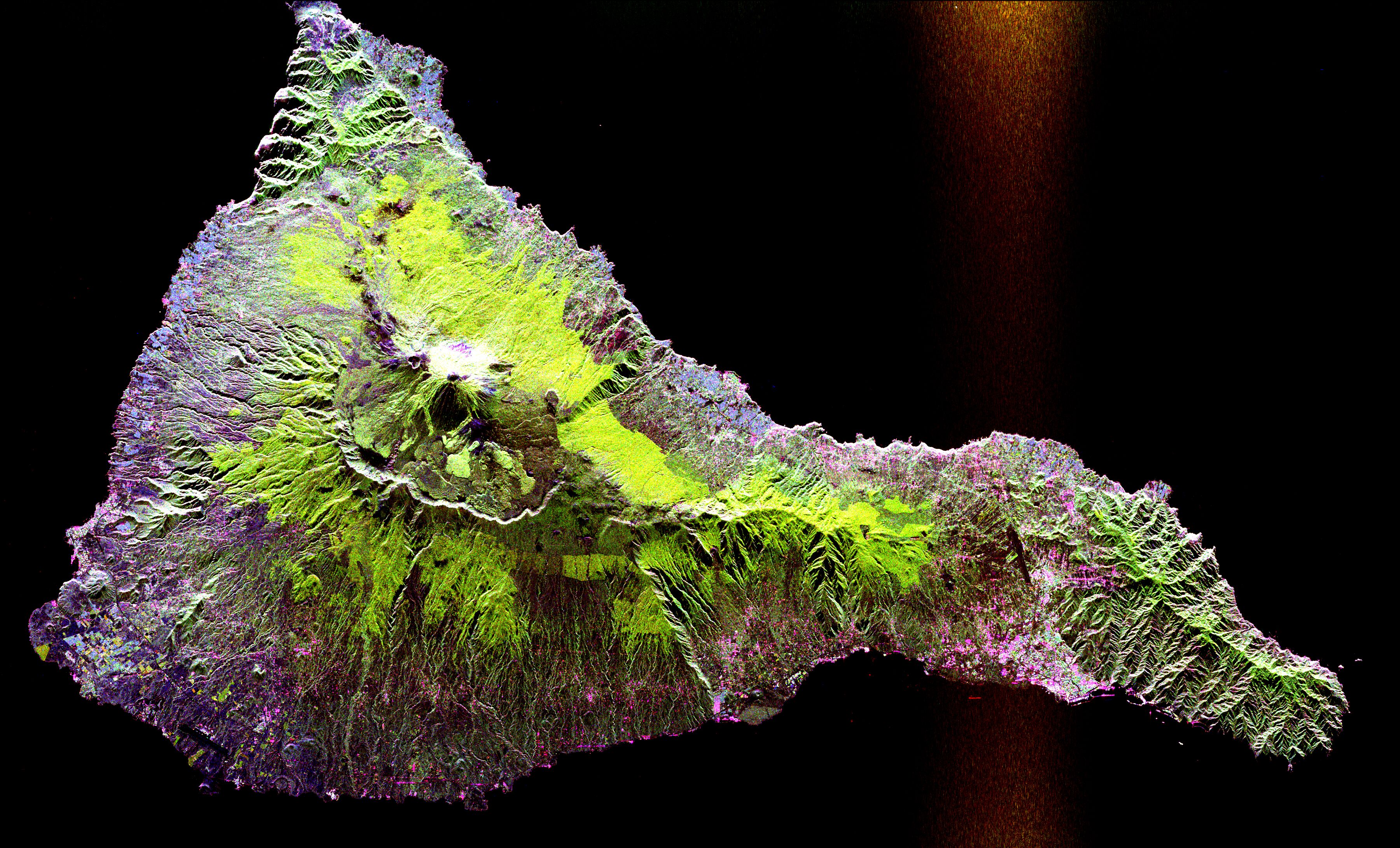
Radar waves have a polarization. Different materials reflect radar waves with different intensities, but anisotropic materials such as grass often reflect different polarizations with different intensities. Some materials will also convert one polarization into another. By emitting a mixture of polarizations and using receiving antennas with a specific polarization, several images can be collected from the same series of pulses. Frequently three such RX-TX polarizations (HH-pol, VV-pol, VH-pol) are used as the three color channels in a synthesized image. This is what has been done in the picture at right. Interpretation of the resulting colors requires significant testing of known materials.

New developments in polarimetry include using the changes in the random polarization returns of some surfaces (such as grass or sand) and between two images of the same location at different times to determine where changes not visible to optical systems occurred. Examples include subterranean tunneling or paths of vehicles driving through the area being imaged. Enhanced SAR sea oil slick observation has been developed by appropriate physical modelling and use of fully polarimetric and dual-polarimetric measurements.

SAR polarimetry

SAR image of Death Valley colored using polarimetry

SAR polarimetry is a technique used for deriving qualitative and quantitative physical information for land, snow and ice, ocean and urban applications based on the measurement and exploration of the polarimetric properties of man-made and natural scatterers. Terrain and land use classification is one of the most important applications of polarimetric synthetic-aperture radar (PolSAR).

SAR polarimetry uses a scattering matrix (S) to identify the scattering behavior of objects after an interaction with electromagnetic wave. The matrix is represented by a combination of horizontal and vertical polarization states of transmitted and received signals.

$S={\begin{bmatrix}S_{HH}&S_{HV}\\S_{VH}&S_{VV}\end{bmatrix}}$

where, HH is for horizontal transmit and horizontal receive, VV is for vertical transmit and vertical receive, HV is for horizontal transmit and vertical receive, and VH – for vertical transmit and horizontal receive.

The first two of these polarization combinations are referred to as like-polarized (or co-polarized), because the transmit and receive polarizations are the same. The last two combinations are referred to as cross-polarized because the transmit and receive polarizations are orthogonal to one another.

Three-component scattering power model

The three-component scattering power model by Freeman and Durden is successfully used for the decomposition of a PolSAR image, applying the reflection symmetry condition using covariance matrix. The method is based on simple physical scattering mechanisms (surface scattering, double-bounce scattering, and volume scattering). The advantage of this scattering model is that it is simple and easy to implement for image processing. There are 2 major approaches for a 3$\times$3 polarimetric matrix decomposition. One is the lexicographic covariance matrix approach based on physically measurable parameters, and the other is the Pauli decomposition which is a coherent decomposition matrix. It represents all the polarimetric information in a single SAR image. The polarimetric information of [S] could be represented by the combination of the intensities $|S_{HH}|^{2},|S_{VV}|^{2},2|S_{HV}|^{2}$ in a single RGB image where all the previous intensities will be coded as a color channel.

Four-component scattering power model

For PolSAR image analysis, there can be cases where reflection symmetry condition does not hold. In those cases a four-component scattering model can be used to decompose polarimetric synthetic-aperture radar (SAR) images. This approach deals with the non-reflection symmetric scattering case. It includes and extends the three-component decomposition method introduced by Freeman and Durden to a fourth component by adding the helix scattering power. This helix power term generally appears in complex urban area but disappears for a natural distributed scatterer.

There is also an improved method using the four-component decomposition algorithm, which was introduced for the general polSAR data image analyses. The SAR data is first filtered which is known as speckle reduction, then each pixel is decomposed by four-component model to determine the surface scattering power ($P_{s}$), double-bounce scattering power ($P_{d}$), volume scattering power ($P_{v}$), and helix scattering power ($P_{c}$). The pixels are then divided into 5 classes (surface, double-bounce, volume, helix, and mixed pixels) classified with respect to maximum powers. A mixed category is added for the pixels having two or three equal dominant scattering powers after computation. The process continues as the pixels in all these categories are divided in 20 small clutter approximately of same number of pixels and merged as desirable, this is called cluster merging. They are iteratively classified and then automatically color is delivered to each class. The summarization of this algorithm leads to an understanding that, brown colors denotes the surface scattering classes, red colors for double-bounce scattering classes, green colors for volume scattering classes, and blue colors for helix scattering classes.

Although this method is aimed for non-reflection case, it automatically includes the reflection symmetry condition, therefore in can be used as a general case. It also preserves the scattering characteristics by taking the mixed scattering category into account therefore proving to be a better algorithm.

Interferometry

Main article: Interferometric synthetic-aperture radar

Rather than discarding the phase data, information can be extracted from it. If two observations of the same terrain from very similar positions are available, aperture synthesis can be performed to provide the resolution performance which would be given by a radar system with dimensions equal to the separation of the two measurements. This technique is called interferometric SAR or InSAR.

If the two samples are obtained simultaneously (perhaps by placing two antennas on the same aircraft, some distance apart), then any phase difference will contain information about the angle from which the radar echo returned. Combining this with the distance information, one can determine the position in three dimensions of the image pixel. In other words, one can extract terrain altitude as well as radar reflectivity, producing a digital elevation model (DEM) with a single airplane pass. One aircraft application at the Canada Centre for Remote Sensing produced digital elevation maps with a resolution of 5 m and altitude errors also about 5 m. Interferometry was used to map many regions of the Earth's surface with unprecedented accuracy using data from the Shuttle Radar Topography Mission.

If the two samples are separated in time, perhaps from two flights over the same terrain, then there are two possible sources of phase shift. The first is terrain altitude, as discussed above. The second is terrain motion: if the terrain has shifted between observations, it will return a different phase. The amount of shift required to cause a significant phase difference is on the order of the wavelength used. This means that if the terrain shifts by centimeters, it can be seen in the resulting image (a digital elevation map must be available to separate the two kinds of phase difference; a third pass may be necessary to produce one).

This second method offers a powerful tool in geology and geography. Glacier flow can be mapped with two passes. Maps showing the land deformation after a minor earthquake or after a volcanic eruption (showing the shrinkage of the whole volcano by several centimeters) have been published.

Differential interferometry

Differential interferometry (D-InSAR) requires taking at least two images with addition of a DEM. The DEM can be either produced by GPS measurements or could be generated by interferometry as long as the time between acquisition of the image pairs is short, which guarantees minimal distortion of the image of the target surface. In principle, 3 images of the ground area with similar image acquisition geometry is often adequate for D-InSar. The principle for detecting ground movement is quite simple. One interferogram is created from the first two images; this is also called the reference interferogram or topographical interferogram. A second interferogram is created that captures topography + distortion. Subtracting the latter from the reference interferogram can reveal differential fringes, indicating movement. The described 3 image D-InSAR generation technique is called 3-pass or double-difference method.

Differential fringes which remain as fringes in the differential interferogram are a result of SAR range changes of any displaced point on the ground from one interferogram to the next. In the differential interferogram, each fringe is directly proportional to the SAR wavelength, which is about 5.6 cm for ERS and RADARSAT single phase cycle. Surface displacement away from the satellite look direction causes an increase in path (translating to phase) difference. Since the signal travels from the SAR antenna to the target and back again, the measured displacement is twice the unit of wavelength. This means in differential interferometry one fringe cycle −Template:Pi to +Template:Pi or one wavelength corresponds to a displacement relative to SAR antenna of only half wavelength (2.8 cm). There are various publications on measuring subsidence movement, slope stability analysis, landslide, glacier movement, etc. tooling D-InSAR. Further advancement to this technique whereby differential interferometry from satellite SAR ascending pass and descending pass can be used to estimate 3-D ground movement. Research in this area has shown accurate measurements of 3-D ground movement with accuracies comparable to GPS based measurements can be achieved.

Tomo-SAR

SAR Tomography is a subfield of a concept named as multi-baseline interferometry. It has been developed to give a 3D exposure to the imaging, which uses the beam formation concept. It can be used when the use demands a focused phase concern between the magnitude and the phase components of the SAR data, during information retrieval. One of the major advantages of Tomo-SAR is that it can separate out the parameters which get scattered, irrespective of how different their motions are. On using Tomo-SAR with differential interferometry, a new combination named "differential tomography" (Diff-Tomo) is developed.

Tomo-SAR has an application based on radar imaging, which is the depiction of Ice Volume and Forest Temporal Coherence (Temporal coherence describes the correlation between waves observed at different moments in time).

Ultra-wideband SAR

Further information: Ultra-wideband

Conventional radar systems emit bursts of radio energy with a fairly narrow range of frequencies. A narrow-band channel, by definition, does not allow rapid changes in modulation. Since it is the change in a received signal that reveals the time of arrival of the signal (obviously an unchanging signal would reveal nothing about "when" it reflected from the target), a signal with only a slow change in modulation cannot reveal the distance to the target as well as a signal with a quick change in modulation.

Ultra-wideband (UWB) refers to any radio transmission that uses a very large bandwidth – which is the same as saying it uses very rapid changes in modulation. Although there is no set bandwidth value that qualifies a signal as "UWB", systems using bandwidths greater than a sizable portion of the center frequency (typically about ten percent, or so) are most often called "UWB" systems. A typical UWB system might use a bandwidth of one-third to one-half of its center frequency. For example, some systems use a bandwidth of about 1 GHz centered around 3 GHz.

There are as many ways to increase the bandwidth of a signal as there are forms of modulation – it is simply a matter of increasing the rate of that modulation. However, the two most common methods used in UWB radar, including SAR, are very short pulses and high-bandwidth chirping. A general description of chirping appears elsewhere in this article. The bandwidth of a chirped system can be as narrow or as wide as the designers desire. Pulse-based UWB systems, being the more common method associated with the term "UWB radar", are described here.

A pulse-based radar system transmits very short pulses of electromagnetic energy, typically only a few waves or less. A very short pulse is, of course, a very rapidly changing signal, and thus occupies a very wide bandwidth. This allows far more accurate measurement of distance, and thus resolution.

The main disadvantage of pulse-based UWB SAR is that the transmitting and receiving front-end electronics are difficult to design for high-power applications. Specifically, the transmit duty cycle is so exceptionally low and pulse time so exceptionally short, that the electronics must be capable of extremely high instantaneous power to rival the average power of conventional radars. (Although it is true that UWB provides a notable gain in channel capacity over a narrow band signal because of the relationship of bandwidth in the Shannon–Hartley theorem and because the low receive duty cycle receives less noise, increasing the signal-to-noise ratio, there is still a notable disparity in link budget because conventional radar might be several orders of magnitude more powerful than a typical pulse-based radar.) So pulse-based UWB SAR is typically used in applications requiring average power levels in the microwatt or milliwatt range, and thus is used for scanning smaller, nearer target areas (several tens of meters), or in cases where lengthy integration (over a span of minutes) of the received signal is possible. Note, however, that this limitation is solved in chirped UWB radar systems.

The principal advantages of UWB radar are better resolution (a few millimeters using commercial off-the-shelf electronics) and more spectral information of target reflectivity.

Doppler-beam sharpening

Doppler Beam Sharpening commonly refers to the method of processing unfocused real-beam phase history to achieve better resolution than could be achieved by processing the real beam without it. Because the real aperture of the radar antenna is so small (compared to the wavelength in use), the radar energy spreads over a wide area (usually many degrees wide in a direction orthogonal (at right angles) to the direction of the platform (aircraft)). Doppler-beam sharpening takes advantage of the motion of the platform in that targets ahead of the platform return a Doppler upshifted signal (slightly higher in frequency) and targets behind the platform return a Doppler downshifted signal (slightly lower in frequency).

The amount of shift varies with the angle forward or backward from the ortho-normal direction. By knowing the speed of the platform, target signal return is placed in a specific angle "bin" that changes over time. Signals are integrated over time and thus the radar "beam" is synthetically reduced to a much smaller aperture – or more accurately (and based on the ability to distinguish smaller Doppler shifts) the system can have hundreds of very "tight" beams concurrently. This technique dramatically improves angular resolution; however, it is far more difficult to take advantage of this technique for range resolution. (See pulse-doppler radar).

Chirped (pulse-compressed) radars

Further information: Chirp

A common technique for many radar systems (usually also found in SAR systems) is to "chirp" the signal. In a "chirped" radar, the pulse is allowed to be much longer. A longer pulse allows more energy to be emitted, and hence received, but usually hinders range resolution. But in a chirped radar, this longer pulse also has a frequency shift during the pulse (hence the chirp or frequency shift). When the "chirped" signal is returned, it must be correlated with the sent pulse. Classically, in analog systems, it is passed to a dispersive delay line (often a surface acoustic wave device) that has the property of varying velocity of propagation based on frequency. This technique "compresses" the pulse in time – thus having the effect of a much shorter pulse (improved range resolution) while having the benefit of longer pulse length (much more signal returned). Newer systems use digital pulse correlation to find the pulse return in the signal.

Typical operation

NASA's AirSAR instrument is attached to the side of a DC-8

In a typical SAR application, a single radar antenna is attached to an aircraft or spacecraft such that a substantial component of the antenna's radiated beam has a wave-propagation direction perpendicular to the flight-path direction. The beam is allowed to be broad in the vertical direction so it will illuminate the terrain from nearly beneath the aircraft out toward the horizon.

Resolution in the range dimension of the image is accomplished by creating pulses which define very short time intervals, either by emitting short pulses consisting of a carrier frequency and the necessary sidebands, all within a certain bandwidth, or by using longer "chirp pulses" in which frequency varies (often linearly) with time within that bandwidth. The differing times at which echoes return allow points at different distances to be distinguished.

SAR antenna of the SAOCOM satellites.

The total signal is that from a beamwidth-sized patch of the ground. To produce a beam that is narrow in the cross-range direction, diffraction effects require that the antenna be wide in that dimension. Therefore, the distinguishing, from each other, of co-range points simply by strengths of returns that persist for as long as they are within the beam width is difficult with aircraft-carryable antennas, because their beams can have linear widths only about two orders of magnitude (hundreds of times) smaller than the range. (Spacecraft-carryable ones can do 10 or more times better.) However, if both the amplitude and the phase of returns are recorded, then the portion of that multi-target return that was scattered radially from any smaller scene element can be extracted by phase-vector correlation of the total return with the form of the return expected from each such element. Careful design and operation can accomplish resolution of items smaller than a millionth of the range, for example, 30 cm at 300 km, or about one foot at nearly 200 miles (320 km).

The process can be thought of as combining the series of spatially distributed observations as if all had been made simultaneously with an antenna as long as the beamwidth and focused on that particular point. The "synthetic aperture" simulated at maximum system range by this process not only is longer than the real antenna, but, in practical applications, it is much longer than the radar aircraft, and tremendously longer than the radar spacecraft.

Image resolution of SAR in its range coordinate (expressed in image pixels per distance unit) is mainly proportional to the radio bandwidth of whatever type of pulse is used. In the cross-range coordinate, the similar resolution is mainly proportional to the bandwidth of the Doppler shift of the signal returns within the beamwidth. Since Doppler frequency depends on the angle of the scattering point's direction from the broadside direction, the Doppler bandwidth available within the beamwidth is the same at all ranges. Hence the theoretical spatial resolution limits in both image dimensions remain constant with variation of range. However, in practice, both the errors that accumulate with data-collection time and the particular techniques used in post-processing further limit cross-range resolution at long ranges.

The conversion of return delay time to geometric range can be very accurate because of the natural constancy of the speed and direction of propagation of electromagnetic waves. However, for an aircraft flying through the never-uniform and never-quiescent atmosphere, the relating of pulse transmission and reception times to successive geometric positions of the antenna must be accompanied by constant adjusting of the return phases to account for sensed irregularities in the flight path. SAR's in spacecraft avoid that atmosphere problem, but still must make corrections for known antenna movements due to rotations of the spacecraft, even those that are reactions to movements of onboard machinery. Locating a SAR in a manned space vehicle may require that the humans carefully remain motionless relative to the vehicle during data collection periods.

Although some references to SARs have characterized them as "radar telescopes", their actual optical analogy is the microscope, the detail in their images being smaller than the length of the synthetic aperture. In radar-engineering terms, while the target area is in the "far field" of the illuminating antenna, it is in the "near field" of the simulated one.

Returns from scatterers within the range extent of any image are spread over a matching time interval. The inter-pulse period must be long enough to allow farthest-range returns from any pulse to finish arriving before the nearest-range ones from the next pulse begin to appear, so that those do not overlap each other in time. On the other hand, the interpulse rate must be fast enough to provide sufficient samples for the desired across-range (or across-beam) resolution. When the radar is to be carried by a high-speed vehicle and is to image a large area at fine resolution, those conditions may clash, leading to what has been called SAR's ambiguity problem. The same considerations apply to "conventional" radars also, but this problem occurs significantly only when resolution is so fine as to be available only through SAR processes. Since the basis of the problem is the information-carrying capacity of the single signal-input channel provided by one antenna, the only solution is to use additional channels fed by additional antennas. The system then becomes a hybrid of a SAR and a phased array, sometimes being called a Vernier array.

Data processing

Combining the series of observations requires significant computational resources, usually using Fourier transform techniques. The high digital computing speed now available allows such processing to be done in near-real time on board a SAR aircraft. (There is necessarily a minimum time delay until all parts of the signal have been received.) The result is a map of radar reflectivity, including both amplitude and phase.

Amplitude data

The amplitude information, when shown in a map-like display, gives information about ground cover in much the same way that a black-and-white photo does. Variations in processing may also be done in either vehicle-borne stations or ground stations for various purposes, so as to accentuate certain image features for detailed target-area analysis.

Phase data

Although the phase information in an image is generally not made available to a human observer of an image display device, it can be preserved numerically, and sometimes allows certain additional features of targets to be recognized.

Coherence speckle

Unfortunately, the phase differences between adjacent image picture elements ("pixels") also produce random interference effects called "coherence speckle", which is a sort of graininess with dimensions on the order of the resolution, causing the concept of resolution to take on a subtly different meaning. This effect is the same as is apparent both visually and photographically in laser-illuminated optical scenes. The scale of that random speckle structure is governed by the size of the synthetic aperture in wavelengths, and cannot be finer than the system's resolution. Speckle structure can be subdued at the expense of resolution.

Optical holography

Before rapid digital computers were available, the data processing was done using an optical holography technique. The analog radar data were recorded as a holographic interference pattern on photographic film at a scale permitting the film to preserve the signal bandwidths (for example, 1:1,000,000 for a radar using a 0.6-meter wavelength). Then light using, for example, 0.6-micrometer waves (as from a helium–neon laser) passing through the hologram could project a terrain image at a scale recordable on another film at reasonable processor focal distances of around a meter. This worked because both SAR and phased arrays are fundamentally similar to optical holography, but using microwaves instead of light waves. The "optical data-processors" developed for this radar purpose were the first effective analog optical computer systems, and were, in fact, devised before the holographic technique was fully adapted to optical imaging. Because of the different sources of range and across-range signal structures in the radar signals, optical data-processors for SAR included not only both spherical and cylindrical lenses, but sometimes conical ones.

Image appearance

The following considerations apply also to real-aperture terrain-imaging radars, but are more consequential when resolution in range is matched to a cross-beam resolution that is available only from a SAR.

Range, cross-range, and angles

The two dimensions of a radar image are range and cross-range. Radar images of limited patches of terrain can resemble oblique photographs, but not ones taken from the location of the radar. This is because the range coordinate in a radar image is perpendicular to the vertical-angle coordinate of an oblique photo. The apparent entrance-pupil position (or camera center) for viewing such an image is therefore not as if at the radar, but as if at a point from which the viewer's line of sight is perpendicular to the slant-range direction connecting radar and target, with slant-range increasing from top to bottom of the image.

Because slant ranges to level terrain vary in vertical angle, each elevation of such terrain appears as a curved surface, specifically a hyperbolic cosine one. Verticals at various ranges are perpendiculars to those curves. The viewer's apparent looking directions are parallel to the curve's "hypcos" axis. Items directly beneath the radar appear as if optically viewed horizontally (i.e., from the side) and those at far ranges as if optically viewed from directly above. These curvatures are not evident unless large extents of near-range terrain, including steep slant ranges, are being viewed.

When viewed as specified above, fine-resolution radar images of small areas can appear most nearly like familiar optical ones, for two reasons. The first reason is easily understood by imagining a flagpole in the scene. The slant-range to its upper end is less than that to its base. Therefore, the pole can appear correctly top-end up only when viewed in the above orientation. Secondly, the radar illumination then being downward, shadows are seen in their most-familiar "overhead-lighting" direction.

Note that the image of the pole's top will overlay that of some terrain point which is on the same slant range arc but at a shorter horizontal range ("ground-range"). Images of scene surfaces which faced both the illumination and the apparent eyepoint will have geometries that resemble those of an optical scene viewed from that eyepoint. However, slopes facing the radar will be foreshortened and ones facing away from it will be lengthened from their horizontal (map) dimensions. The former will therefore be brightened and the latter dimmed.

Returns from slopes steeper than perpendicular to slant range will be overlaid on those of lower-elevation terrain at a nearer ground-range, both being visible but intermingled. This is especially the case for vertical surfaces like the walls of buildings. Another viewing inconvenience that arises when a surface is steeper than perpendicular to the slant range is that it is then illuminated on one face but "viewed" from the reverse face. Then one "sees", for example, the radar-facing wall of a building as if from the inside, while the building's interior and the rear wall (that nearest to, hence expected to be optically visible to, the viewer) have vanished, since they lack illumination, being in the shadow of the front wall and the roof. Some return from the roof may overlay that from the front wall, and both of those may overlay return from terrain in front of the building. The visible building shadow will include those of all illuminated items. Long shadows may exhibit blurred edges due to the illuminating antenna's movement during the "time exposure" needed to create the image.

Mirroring artefacts and shadows

Surfaces that we usually consider rough will, if that roughness consists of relief less than the radar wavelength, behave as smooth mirrors, showing, beyond such a surface, additional images of items in front of it. Those mirror images will appear within the shadow of the mirroring surface, sometimes filling the entire shadow, thus preventing recognition of the shadow.

An important fact that applies to SARs but not to real-aperture radars is that the direction of overlay of any scene point is not directly toward the radar, but toward that point of the SAR's current path direction that is nearest to the target point. If the SAR is "squinting" forward or aft away from the exactly broadside direction, then the illumination direction, and hence the shadow direction, will not be opposite to the overlay direction, but slanted to right or left from it. An image will appear with the correct projection geometry when viewed so that the overlay direction is vertical, the SAR's flight-path is above the image, and range increases somewhat downward.

Objects in motion

Objects in motion within a SAR scene alter the Doppler frequencies of the returns. Such objects therefore appear in the image at locations offset in the across-range direction by amounts proportional to the range-direction component of their velocity. Road vehicles may be depicted off the roadway and therefore not recognized as road traffic items. Trains appearing away from their tracks are more easily properly recognized by their length parallel to known trackage as well as by the absence of an equal length of railbed signature and of some adjacent terrain, both having been shadowed by the train. While images of moving vessels can be offset from the line of the earlier parts of their wakes, the more recent parts of the wake, which still partake of some of the vessel's motion, appear as curves connecting the vessel image to the relatively quiescent far-aft wake. In such identifiable cases, speed and direction of the moving items can be determined from the amounts of their offsets. The along-track component of a target's motion causes some defocus. Random motions such as that of wind-driven tree foliage, vehicles driven over rough terrain, or humans or other animals walking or running generally render those items not focusable, resulting in blurring or even effective invisibility.

These considerations, along with the speckle structure due to coherence, take some getting used to in order to correctly interpret SAR images. To assist in that, large collections of significant target signatures have been accumulated by performing many test flights over known terrains and cultural objects.

History

See also: Aperture synthesis § History

Carl A. Wiley, a mathematician at Goodyear Aircraft Company in Litchfield Park, Arizona, invented synthetic aperture radar in June 1951 while working on a correlation guidance system for the Atlas ICBM program. In early 1952, Wiley, together with Fred Heisley and Bill Welty, constructed a concept validation system known as DOUSER ("Doppler Unbeamed Search Radar"). During the 1950s and 1960s, Goodyear Aircraft (later Goodyear Aerospace) introduced numerous advancements in SAR technology, many with the help from Don Beckerleg.

Independently of Wiley's work, experimental trials in early 1952 by Sherwin and others at the University of Illinois' Control Systems Laboratory showed results that they pointed out "could provide the basis for radar systems with greatly improved angular resolution" and might even lead to systems capable of focusing at all ranges simultaneously.

In both of those programs, processing of the radar returns was done by electrical-circuit filtering methods. In essence, signal strength in isolated discrete bands of Doppler frequency defined image intensities that were displayed at matching angular positions within proper range locations. When only the central (zero-Doppler band) portion of the return signals was used, the effect was as if only that central part of the beam existed. That led to the term Doppler Beam Sharpening. Displaying returns from several adjacent non-zero Doppler frequency bands accomplished further "beam-subdividing" (sometimes called "unfocused radar", though it could have been considered "semi-focused"). Wiley's patent, applied for in 1954, still proposed similar processing. The bulkiness of the circuitry then available limited the extent to which those schemes might further improve resolution.

The principle was included in a memorandum authored by Walter Hausz of General Electric that was part of the then-secret report of a 1952 Dept. of Defense summer study conference called TEOTA ("The Eyes of the Army"), which sought to identify new techniques useful for military reconnaissance and technical gathering of intelligence. A follow-on summer program in 1953 at the University of Michigan, called Project Wolverine, identified several of the TEOTA subjects, including Doppler-assisted sub-beamwidth resolution, as research efforts to be sponsored by the Department of Defense (DoD) at various academic and industrial research laboratories. In that same year, the Illinois group produced a "strip-map" image exhibiting a considerable amount of sub-beamwidth resolution.

A more advanced focused-radar project was among several remote sensing schemes assigned in 1953 to Project Michigan, a tri-service-sponsored (Army, Navy, Air Force) program at the University of Michigan's Willow Run Research Center (WRRC), that program being administered by the Army Signal Corps. Initially called the side-looking radar project, it was carried out by a group first known as the Radar Laboratory and later as the Radar and Optics Laboratory. It proposed to take into account, not just the short-term existence of several particular Doppler shifts, but the entire history of the steadily varying shifts from each target as the latter crossed the beam. An early analysis by Dr. Louis J. Cutrona, Weston E. Vivian, and Emmett N. Leith of that group showed that such a fully focused system should yield, at all ranges, a resolution equal to the width (or, by some criteria, the half-width) of the real antenna carried on the radar aircraft and continually pointed broadside to the aircraft's path.

The required data processing amounted to calculating cross-correlations of the received signals with samples of the forms of signals to be expected from unit-amplitude sources at the various ranges. At that time, even large digital computers had capabilities somewhat near the levels of today's four-function handheld calculators, hence were nowhere near able to do such a huge amount of computation. Instead, the device for doing the correlation computations was to be an optical correlator.

It was proposed that signals received by the traveling antenna and coherently detected be displayed as a single range-trace line across the diameter of the face of a cathode-ray tube, the line's successive forms being recorded as images projected onto a film traveling perpendicular to the length of that line. The information on the developed film was to be subsequently processed in the laboratory on equipment still to be devised as a principal task of the project. In the initial processor proposal, an arrangement of lenses was expected to multiply the recorded signals point-by-point with the known signal forms by passing light successively through both the signal film and another film containing the known signal pattern. The subsequent summation, or integration, step of the correlation was to be done by converging appropriate sets of multiplication products by the focusing action of one or more spherical and cylindrical lenses. The processor was to be, in effect, an optical analog computer performing large-scale scalar arithmetic calculations in many channels (with many light "rays") at once. Ultimately, two such devices would be needed, their outputs to be combined as quadrature components of the complete solution.

Fortunately (as it turned out), a desire to keep the equipment small had led to recording the reference pattern on 35 mm film. Trials promptly showed that the patterns on the film were so fine as to show pronounced diffraction effects that prevented sharp final focusing.

That led Leith, a physicist who was devising the correlator, to recognize that those effects in themselves could, by natural processes, perform a significant part of the needed processing, since along-track strips of the recording operated like diametrical slices of a series of circular optical zone plates. Any such plate performs somewhat like a lens, each plate having a specific focal length for any given wavelength. The recording that had been considered as scalar became recognized as pairs of opposite-sign vector ones of many spatial frequencies plus a zero-frequency "bias" quantity. The needed correlation summation changed from a pair of scalar ones to a single vector one.

Each zone plate strip has two equal but oppositely signed focal lengths, one real, where a beam through it converges to a focus, and one virtual, where another beam appears to have diverged from, beyond the other face of the zone plate. The zero-frequency (DC bias) component has no focal point, but overlays both the converging and diverging beams. The key to obtaining, from the converging wave component, focused images that are not overlaid with unwanted haze from the other two is to block the latter, allowing only the wanted beam to pass through a properly positioned frequency-band selecting aperture.

Each radar range yields a zone plate strip with a focal length proportional to that range. This fact became a principal complication in the design of optical processors. Consequently, technical journals of the time contain a large volume of material devoted to ways for coping with the variation of focus with range.

For that major change in approach, the light used had to be both monochromatic and coherent, properties that were already a requirement on the radar radiation. Lasers also then being in the future, the best then-available approximation to a coherent light source was the output of a mercury vapor lamp, passed through a color filter that was matched to the lamp spectrum's green band, and then concentrated as well as possible onto a very small beam-limiting aperture. While the resulting amount of light was so weak that very long exposure times had to be used, a workable optical correlator was assembled in time to be used when appropriate data became available.

Although creating that radar was a more straightforward task based on already-known techniques, that work did demand the achievement of signal linearity and frequency stability that were at the extreme state of the art. An adequate instrument was designed and built by the Radar Laboratory and was installed in a C-46 (Curtiss Commando) aircraft. Because the aircraft was bailed to WRRC by the U. S. Army and was flown and maintained by WRRC's own pilots and ground personnel, it was available for many flights at times matching the Radar Laboratory's needs, a feature important for allowing frequent re-testing and "debugging" of the continually developing complex equipment. By contrast, the Illinois group had used a C-46 belonging to the Air Force and flown by AF pilots only by pre-arrangement, resulting, in the eyes of those researchers, in limitation to a less-than-desirable frequency of flight tests of their equipment, hence a low bandwidth of feedback from tests. (Later work with newer Convair aircraft continued the Michigan group's local control of flight schedules.)

Michigan's chosen 5-foot (1.5 m)-wide World War II-surplus antenna was theoretically capable of 5-foot (1.5 m) resolution, but data from only 10% of the beamwidth was used at first, the goal at that time being to demonstrate 50-foot (15 m) resolution. It was understood that finer resolution would require the added development of means for sensing departures of the aircraft from an ideal heading and flight path, and for using that information for making needed corrections to the antenna pointing and to the received signals before processing. After numerous trials in which even small atmospheric turbulence kept the aircraft from flying straight and level enough for good 50-foot (15 m) data, one pre-dawn flight in August 1957 yielded a map-like image of the Willow Run Airport area which did demonstrate 50-foot (15 m) resolution in some parts of the image, whereas the illuminated beam width there was 900 feet (270 m). Although the program had been considered for termination by DoD due to what had seemed to be a lack of results, that first success ensured further funding to continue development leading to solutions to those recognized needs.

First successful focussed airborne synthetic aperture radar image, Willow Run Airport and vicinity, August 1957. Image courtesy University of Michigan.

The SAR principle was first acknowledged publicly via an April 1960 press release about the U. S. Army experimental AN/UPD-1 system, which consisted of an airborne element made by Texas Instruments and installed in a Beech L-23D aircraft and a mobile ground data-processing station made by WRRC and installed in a military van. At the time, the nature of the data processor was not revealed. A technical article in the journal of the IRE (Institute of Radio Engineers) Professional Group on Military Electronics in February 1961 described the SAR principle and both the C-46 and AN/UPD-1 versions, but did not tell how the data were processed, nor that the UPD-1's maximum resolution capability was about 50 feet (15 m). However, the June 1960 issue of the IRE Professional Group on Information Theory had contained a long article on "Optical Data Processing and Filtering Systems" by members of the Michigan group. Although it did not refer to the use of those techniques for radar, readers of both journals could quite easily understand the existence of a connection between articles sharing some authors.

An operational system to be carried in a reconnaissance version of the F-4 "Phantom" aircraft was quickly devised and was used briefly in Vietnam, where it failed to favorably impress its users, due to the combination of its low resolution (similar to the UPD-1's), the speckly nature of its coherent-wave images (similar to the speckliness of laser images), and the poorly understood dissimilarity of its range/cross-range images from the angle/angle optical ones familiar to military photo interpreters. The lessons it provided were well learned by subsequent researchers, operational system designers, image-interpreter trainers, and the DoD sponsors of further development and acquisition.

In subsequent work the technique's latent capability was eventually achieved. That work, depending on advanced radar circuit designs and precision sensing of departures from ideal straight flight, along with more sophisticated optical processors using laser light sources and specially designed very large lenses made from remarkably clear glass, allowed the Michigan group to advance system resolution, at about 5-year intervals, first to 15 feet (4.6 m), then 5 feet (1.5 m), and, by the mid-1970s, to 1 foot (the latter only over very short range intervals while processing was still being done optically). The latter levels and the associated very wide dynamic range proved suitable for identifying many objects of military concern as well as soil, water, vegetation, and ice features being studied by a variety of environmental researchers having security clearances allowing them access to what was then classified imagery. Similarly improved operational systems soon followed each of those finer-resolution steps.

Comparison of earliest SAR image with a later improved-resolution one. Additionally, the data-processing light source had been changed from a mercury lamp to a laser. Image data courtesy of University of Michigan and Natural Resources Canada.

Even the 5-foot (1.5 m) resolution stage had over-taxed the ability of cathode-ray tubes (limited to about 2000 distinguishable items across the screen diameter) to deliver fine enough details to signal films while still covering wide range swaths, and taxed the optical processing systems in similar ways. However, at about the same time, digital computers finally became capable of doing the processing without similar limitation, and the consequent presentation of the images on cathode ray tube monitors instead of film allowed for better control over tonal reproduction and for more convenient image mensuration.

Achievement of the finest resolutions at long ranges was aided by adding the capability to swing a larger airborne antenna so as to more strongly illuminate a limited target area continually while collecting data over several degrees of aspect, removing the previous limitation of resolution to the antenna width. This was referred to as the spotlight mode, which no longer produced continuous-swath images but, instead, images of isolated patches of terrain.

It was understood very early in SAR development that the extremely smooth orbital path of an out-of-the-atmosphere platform made it ideally suited to SAR operation. Early experience with artificial earth satellites had also demonstrated that the Doppler frequency shifts of signals traveling through the ionosphere and atmosphere were stable enough to permit very fine resolution to be achievable even at ranges of hundreds of kilometers. The first spaceborne SAR images of Earth were demonstrated by a project now referred to as Quill (declassified in 2012).

After the initial work began, several of the capabilities for creating useful classified systems did not exist for another two decades. That seemingly slow rate of advances was often paced by the progress of other inventions, such as the laser, the digital computer, circuit miniaturization, and compact data storage. Once the laser appeared, optical data processing became a fast process because it provided many parallel analog channels, but devising optical chains suited to matching signal focal lengths to ranges proceeded by many stages and turned out to call for some novel optical components. Since the process depended on diffraction of light waves, it required anti-vibration mountings, clean rooms, and highly trained operators. Even at its best, its use of CRTs and film for data storage placed limits on the range depth of images.

At several stages, attaining the frequently over-optimistic expectations for digital computation equipment proved to take far longer than anticipated. For example, the SEASAT system was ready to orbit before its digital processor became available, so a quickly assembled optical recording and processing scheme had to be used to obtain timely confirmation of system operation. In 1978, the first digital SAR processor was developed by the Canadian aerospace company MacDonald Dettwiler (MDA). When its digital processor was finally completed and used, the digital equipment of that time took many hours to create one swath of image from each run of a few seconds of data. Still, while that was a step down in speed, it was a step up in image quality. Modern methods now provide both high speed and high quality.

Although the above specifies the system development contributions of only a few organizations, many other groups had also become players as the value of SAR became more and more apparent. Especially crucial to the organization and funding of the initial long development process was the technical expertise and foresight of a number of both civilian and uniformed project managers in equipment procurement agencies in the federal government, particularly, of course, ones in the armed forces and in the intelligence agencies, and also in some civilian space agencies.

Since a number of publications and Internet sites refer to a young MIT physics graduate named Robert Rines as having invented fine-resolution radar in the 1940s, persons who have been exposed to those may wonder why that has not been mentioned here. Actually, none of his several radar-image-related patents actually had that goal. Instead, they presumed that fine-resolution images of radar object fields could be accomplished by already-known "dielectric lenses", the inventive parts of those patents being ways to convert those microwave-formed images to visible ones. However, that presumption incorrectly implied that such lenses and their images could be of sizes comparable to their optical-wave counterparts, whereas the tremendously larger wavelengths of microwaves would actually require the lenses to have apertures thousands of feet (or meters) wide, like the ones simulated by SARs, and the images would be comparably large. Apparently not only did that inventor fail to recognize that fact, but so also did the patent examiners who approved his several applications, and so also have those who have propagated the erroneous tale so widely. Persons seeking to understand SAR should not be misled by references to those patents.

Data collection

A model of a German SAR-Lupe reconnaissance satellite inside a Cosmos-3M rocket.

Highly accurate data can be collected by aircraft overflying the terrain in question. In the 1980s, as a prototype for instruments to be flown on the NASA Space Shuttles, NASA operated a synthetic aperture radar on a NASA Convair 990. In 1986, this plane caught fire on takeoff. In 1988, NASA rebuilt a C, L, and P-band SAR to fly on the NASA DC-8 aircraft. Called AIRSAR, it flew missions at sites around the world until 2004. Another such aircraft, the Convair 580, was flown by the Canada Center for Remote Sensing until about 1996 when it was handed over to Environment Canada due to budgetary reasons. Most land-surveying applications are now carried out by satellite observation. Satellites such as ERS-1/2, JERS-1, Envisat ASAR, and RADARSAT-1 were launched explicitly to carry out this sort of observation. Their capabilities differ, particularly in their support for interferometry, but all have collected tremendous amounts of valuable data. The Space Shuttle also carried synthetic aperture radar equipment during the SIR-A and SIR-B missions during the 1980s, the Shuttle Radar Laboratory (SRL) missions in 1994 and the Shuttle Radar Topography Mission in 2000.

The Venera 15 and Venera 16 followed later by the Magellan space probe mapped the surface of Venus over several years using synthetic aperture radar.

Titan – Evolving feature in Ligeia Mare (SAR; 21 August 2014).

Synthetic aperture radar was first used by NASA on JPL's Seasat oceanographic satellite in 1978 (this mission also carried an altimeter and a scatterometer); it was later developed more extensively on the Spaceborne Imaging Radar (SIR) missions on the space shuttle in 1981, 1984 and 1994. The Cassini mission to Saturn used SAR to map the surface of the planet's major moon Titan, whose surface is partly hidden from direct optical inspection by atmospheric haze. The SHARAD sounding radar on the Mars Reconnaissance Orbiter and MARSIS instrument on Mars Express have observed bedrock beneath the surface of the Mars polar ice and also indicated the likelihood of substantial water ice in the Martian middle latitudes. The Lunar Reconnaissance Orbiter, launched in 2009, carries a SAR instrument called Mini-RF, which was designed largely to look for water ice deposits on the poles of the Moon.

Titan – Ligeia Mare – SAR and clearer despeckled views.

The Mineseeker Project is designing a system for determining whether regions contain landmines based on a blimp carrying ultra-wideband synthetic aperture radar. Initial trials show promise; the radar is able to detect even buried plastic mines.

SAR has been used in radio astronomy for many years to simulate a large radio telescope by combining observations taken from multiple locations using a mobile antenna.

The National Reconnaissance Office maintains a fleet of (now declassified) synthetic aperture radar satellites commonly designated as Lacrosse or Onyx.

In February 2009, the Sentinel R1 surveillance aircraft entered service in the RAF, equipped with the SAR-based Airborne Stand-Off Radar (ASTOR) system.

The German Armed Forces' (Bundeswehr) military SAR-Lupe reconnaissance satellite system has been fully operational since 22 July 2008.

As of January 2021, multiple commercial companies have started launching constellations of satellites for collecting SAR imagery of Earth.

Data distribution

The Alaska Satellite Facility provides production, archiving and distribution to the scientific community of SAR data products and tools from active and past missions, including the June 2013 release of newly processed, 35-year-old Seasat SAR imagery.

The Center for Southeastern Tropical Advanced Remote Sensing (CSTARS) downlinks and processes SAR data (as well as other data) from a variety of satellites and supports the University of Miami Rosenstiel School of Marine and Atmospheric Science. CSTARS also supports disaster relief operations, oceanographic and meteorological research, and port and maritime security research projects.

Relationship to phased arrays

Further information: Phased array

A technique closely related to SAR uses an array (referred to as a "phased array") of real antenna elements spatially distributed over either one or two dimensions perpendicular to the radar-range dimension. These physical arrays are truly synthetic ones, indeed being created by synthesis of a collection of subsidiary physical antennas. Their operation need not involve motion relative to targets. All elements of these arrays receive simultaneously in real time, and the signals passing through them can be individually subjected to controlled shifts of the phases of those signals. One result can be to respond most strongly to radiation received from a specific small scene area, focusing on that area to determine its contribution to the total signal received. The coherently detected set of signals received over the entire array aperture can be replicated in several data-processing channels and processed differently in each. The set of responses thus traced to different small scene areas can be displayed together as an image of the scene.

In comparison, a SAR's (commonly) single physical antenna element gathers signals at different positions at different times. When the radar is carried by an aircraft or an orbiting vehicle, those positions are functions of a single variable, distance along the vehicle's path, which is a single mathematical dimension (not necessarily the same as a linear geometric dimension). The signals are stored, thus becoming functions, no longer of time, but of recording locations along that dimension. When the stored signals are read out later and combined with specific phase shifts, the result is the same as if the recorded data had been gathered by an equally long and shaped phased array. What is thus synthesized is a set of signals equivalent to what could have been received simultaneously by such an actual large-aperture (in one dimension) phased array. The SAR simulates (rather than synthesizes) that long one-dimensional phased array. Although the term in the title of this article has thus been incorrectly derived, it is now firmly established by half a century of usage.

While operation of a phased array is readily understood as a completely geometric technique, the fact that a synthetic aperture system gathers its data as it (or its target) moves at some speed means that phases which varied with the distance traveled originally varied with time, hence constituted temporal frequencies. Temporal frequencies being the variables commonly used by radar engineers, their analyses of SAR systems are usually (and very productively) couched in such terms. In particular, the variation of phase during flight over the length of the synthetic aperture is seen as a sequence of Doppler shifts of the received frequency from that of the transmitted frequency. It is significant, though, to realize that, once the received data have been recorded and thus have become timeless, the SAR data-processing situation is also understandable as a special type of phased array, treatable as a completely geometric process.

The core of both the SAR and the phased array techniques is that the distances that radar waves travel to and back from each scene element consist of some integer number of wavelengths plus some fraction of a "final" wavelength. Those fractions cause differences between the phases of the re-radiation received at various SAR or array positions. Coherent detection is needed to capture the signal phase information in addition to the signal amplitude information. That type of detection requires finding the differences between the phases of the received signals and the simultaneous phase of a well-preserved sample of the transmitted illumination.

Every wave scattered from any point in the scene has a circular curvature about that point as a center. Signals from scene points at different ranges therefore arrive at a planar array with different curvatures, resulting in signal phase changes which follow different quadratic variations across a planar phased array. Additional linear variations result from points located in different directions from the center of the array. Fortunately, any one combination of these variations is unique to one scene point, and is calculable. For a SAR, the two-way travel doubles that phase change.

In reading the following two paragraphs, be particularly careful to distinguish between array elements and scene elements. Also, each of the latter has a matching image element.

Comparison of the array-signal phase variation across the array with the total calculated phase variation pattern can reveal the relative portion of the total received signal that came from the only scene point that could be responsible for that pattern. One way to do the comparison is by a correlation computation, multiplying, for each scene element, the received and the calculated field-intensity values array element by array element and then summing the products for each scene element. Alternatively, one could, for each scene element, subtract each array element's calculated phase shift from the actual received phase and then vectorially sum the resulting field-intensity differences over the array. Wherever in the scene the two phases substantially cancel everywhere in the array, the difference vectors being added are in phase, yielding, for that scene point, a maximum value for the sum.

The equivalence of these two methods can be seen by recognizing that multiplication of sinusoids can be done by summing phases which are complex-number exponents of e, the base of natural logarithms.

However it is done, the image-deriving process amounts to "backtracking" the process by which nature previously spread the scene information over the array. In each direction, the process may be viewed as a Fourier transform, which is a type of correlation process. The image-extraction process we use can then be seen as another Fourier transform which is a reversal of the original natural one.

It is important to realize that only those sub-wavelength differences of successive ranges from the transmitting antenna to each target point and back, which govern signal phase, are used to refine the resolution in any geometric dimension. The central direction and the angular width of the illuminating beam do not contribute directly to creating that fine resolution. Instead, they serve only to select the solid-angle region from which usable range data are received. While some distinguishing of the ranges of different scene items can be made from the forms of their sub-wavelength range variations at short ranges, the very large depth of focus that occurs at long ranges usually requires that over-all range differences (larger than a wavelength) be used to define range resolutions comparable to the achievable cross-range resolution.

See also

• Alaska Satellite Facility
• Aperture synthesis
• Beamforming
• Earth observation satellite
• High Resolution Wide Swath SAR imaging
• Interferometric synthetic aperture radar (InSAR)
• Inverse synthetic aperture radar (ISAR)
• Magellan space probe
• Pulse-Doppler radar
• Radar MASINT
• Remote sensing
• SAR Lupe
• Seasat
• Sentinel-1
• Speckle noise
• Synthetic aperture sonar
• Synthetic Aperture Ultrasound
• Synthetic array heterodyne detection (SAHD)
• Synthetically thinned aperture radar
• TerraSAR-X
• Terrestrial SAR Interferometry (TInSAR)
• Very Long Baseline Interferometry (VLBI)
• Wave radar

External links

• InSAR measurements from the Space Shuttle
• Images from the Space Shuttle SAR instrument
• The Alaska Satellite Facility has numerous technical documents, including an introductory text on SAR theory and scientific applications
• SAR Journal SAR Journal tracks the Synthetic Aperture Radar (SAR) industry
• NASA radar reveals hidden remains at ancient Angkor – Jet Propulsion Laboratory