.svg)
File:LimSup.png
Size of this preview: 220 × 112 pixels. Other resolutions: 320 × 164 pixels | 500 × 256 pixels | 996 × 509 pixels.
Original file (996 × 509 pixels, file size: 46 KB, MIME type: image/png)
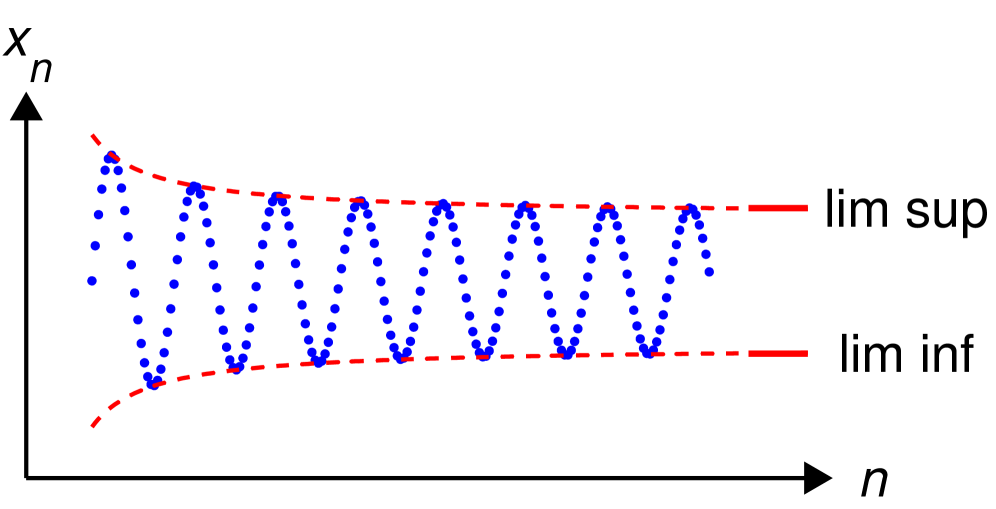
Summary
Made by myself with matlab.

|
File:LimSup.svg is a vector version of this file. It should be used in place of this PNG file when not inferior.
File:LimSup.png → File:LimSup.svg
For more information, see Help:SVG. |
 |
Licensing
| I, the copyright holder of this work, release this work into the public domain. This applies worldwide. In some countries this may not be legally possible; if so: I grant anyone the right to use this work for any purpose, without any conditions, unless such conditions are required by law. |
Source code (MATLAB)
function main() % draw an illustration for limit superior and limit inferior

% prepare the screen and define some parameters
clf; hold on; axis equal; axis off;
fontsize=25; thick_line=3; thin_line=2;
black=[0, 0, 0]; red=[1, 0, 0]; blue=[0, 0, 1];
arrowsize=0.5; arrow_type=1; arrow_angle=30; % (angle in degrees)
circrad=0.07; % radius of ball showing up in places


B=9.4;
X=0:0.05:B;

f=inline('(X+2)./(X+0.9)', 'X');
Y=sin(5*X).*f(X);

for i=1:length(X)
   ball(X(i), Y(i), circrad, blue);
end

K=1.5;
X=0:0.05:(B+K);
Z=f(X);
plot(X, Z, 'r--', 'linewidth', thin_line)
plot(X, -Z, 'r--', 'linewidth', thin_line)

L=f(B);
plot([B+0.4*K B+K], [L, L], 'linestyle', '-', 'linewidth', thick_line, 'color', red);
plot([B+0.4*K B+K], [-L, -L], 'linestyle', '-', 'linewidth', thick_line, 'color', red);

shift=2*K;
H=text(B+shift, L,  'lim sup');          set(H, 'fontsize', fontsize, 'HorizontalAlignment', 'c')
H=text(B+shift, -L,  'lim inf');          set(H, 'fontsize', fontsize, 'HorizontalAlignment', 'c')

shift=-3;
K1=1.2; K2=2.6;
arrow([-1 shift], [K1*B, shift],          thin_line, arrowsize, arrow_angle, arrow_type, black)
arrow([-1, shift], [-1, K2*L],            thin_line, arrowsize, arrow_angle, arrow_type, black)

axis ([-0.2*B, K1*B+1, -2*L+shift, K2*L]);

H=text(K1*B+0.6, shift,  '\it{n}');          set(H, 'fontsize', fontsize, 'HorizontalAlignment', 'c')
H=text(-1, K2*L+0.5,  '\it{x_n}');          set(H, 'fontsize', fontsize, 'HorizontalAlignment', 'c')

saveas(gcf, 'LimSup.eps', 'psc2') % export to eps

function ball(x, y, r, color)
   Theta=0:0.1:2*pi;
   X=r*cos(Theta)+x;
   Y=r*sin(Theta)+y;
   H=fill(X, Y, color);
   set(H, 'EdgeColor', 'none');


function arrow(start, stop, thickness, arrow_size, sharpness, arrow_type, color)

% Function arguments:
% start, stop:  start and end coordinates of arrow, vectors of size 2
% thickness:    thickness of arrow stick
% arrow_size:   the size of the two sides of the angle in this picture ->
% sharpness:    angle between the arrow stick and arrow side, in degrees
% arrow_type:   1 for filled arrow, otherwise the arrow will be just two segments
% color:        arrow color, a vector of length three with values in [0, 1]

% convert to complex numbers
   i=sqrt(-1);
   start=start(1)+i*start(2); stop=stop(1)+i*stop(2);
   rotate_angle=exp(i*pi*sharpness/180);

% points making up the arrow tip (besides the "stop" point)
   point1 = stop - (arrow_size*rotate_angle)*(stop-start)/abs(stop-start);
   point2 = stop - (arrow_size/rotate_angle)*(stop-start)/abs(stop-start);

   if arrow_type==1 % filled arrow

      % plot the stick, but not till the end, looks bad
      t=0.5*arrow_size*cos(pi*sharpness/180)/abs(stop-start); stop1=t*start+(1-t)*stop;
      plot(real([start, stop1]), imag([start, stop1]), 'LineWidth', thickness, 'Color', color);

      % fill the arrow
      H=fill(real([stop, point1, point2]), imag([stop, point1, point2]), color);
      set(H, 'EdgeColor', 'none')

   else % two-segment arrow
      plot(real([start, stop]), imag([start, stop]),   'LineWidth', thickness, 'Color', color);
      plot(real([stop, point1]), imag([stop, point1]), 'LineWidth', thickness, 'Color', color);
      plot(real([stop, point2]), imag([stop, point2]), 'LineWidth', thickness, 'Color', color);
   end
File history
Click on a date/time to view the file as it appeared at that time.
| Date/Time | Thumbnail | Dimensions | User | Comment | |
|---|---|---|---|---|---|
| current | 22:32, 24 February 2007 | | 996 × 509 (46 KB) | wikimediacommons>Oleg Alexandrov | Made by myself with matlab. |
File usage
The following page uses this file: